Exercises

Create a model of a simple heat pump using R290 as refrigerant and with the boundary conditions denoted in table below. Do not consider hot side of the evaporator or cold side of the condenser in your model.

Fig. 9 Flow sheet of the simple heat pump.

Setup

Location	Parameter	Value	Unit
2	Temperature	10	°C
4	Temperature	60	°C
Condenser	Heat transfer	1	MW
Compressor	efficiency	80	%

Tasks part 1

Calculate:

• pressure levels for evaporation and condensation.

• COP and compressor power input.

• the Carnot factor.

• the mass flow of the refrigerant.

Create three figures:

• A logph-diagram of the cycle.

• Two diagrams indicating the dependency of the COP:

  • as function of the heat temperature level

  • as function of the heat sink temperature level

We can calculate the evaporator and condenser outlet state based on temperature specification. The isentropic efficiency value allows us to calculate the compressor outlet enthalpy. Finally, the condenser heat production leads to the mass flow.

from CoolProp.CoolProp import PropsSI



fluid = "R290"
t_2 = 283.15
t_4 = 333.15
eta_s = 0.8
heat = -1e6

p_2 = PropsSI("P", "T", t_2, "Q", 1, fluid)
p_4 = PropsSI("P", "T", t_4, "Q", 0, fluid)

h_2 = PropsSI("H", "T", t_2, "Q", 1, fluid)
s_2 = PropsSI("S", "T", t_2, "Q", 1, fluid)

p_3 = p_4
h_3s = PropsSI("H", "S", s_2, "P", p_3, fluid)
h_3 = h_2 + (h_3s - h_2) / eta_s

h_4 = PropsSI("H", "T", t_4, "Q", 0, fluid)
h_1 = h_4
p_1 = p_2

m = heat / (h_4 - h_3)
power = m * (h_3 - h_2)
cop = abs(heat) / power
heat_evap = abs(heat) - power

We can examine a couple of the results calculated:

round(cop, 2)

4.13

round(heat_evap)

757702

round(power)

242298

round(m, 2)

3.48

round(p_2)

636602

round(p_4)

2116753

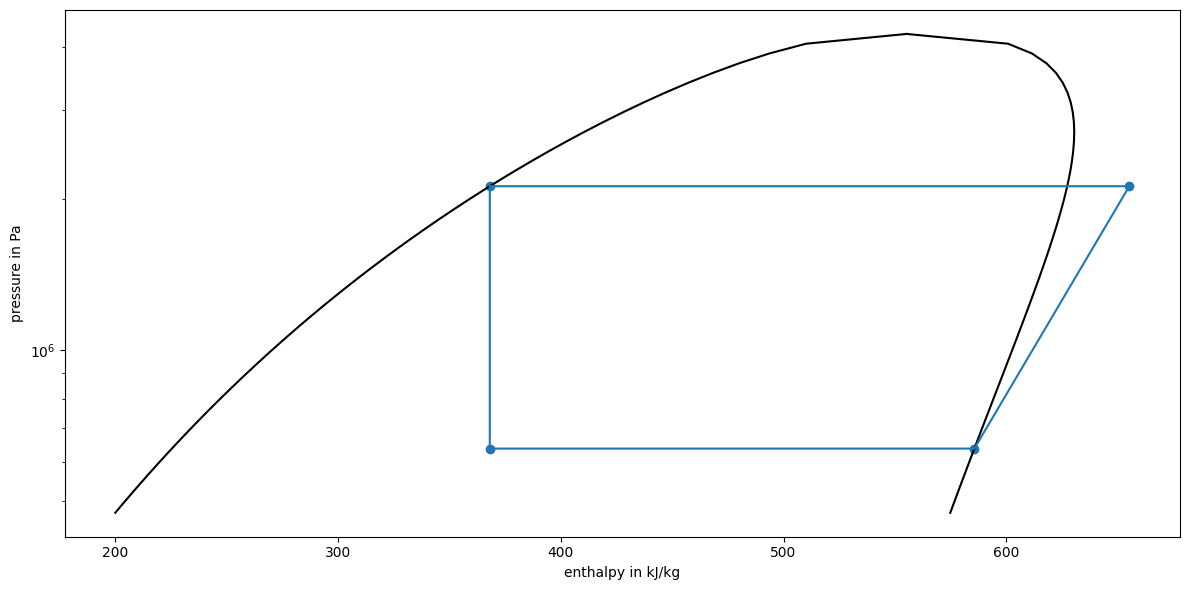
Next we create a logph-diagram of the process. For that, we start by plotting the saturation dome and then insert the states and connect them.

import numpy as np
from matplotlib import pyplot as plt


p_range = np.geomspace(PropsSI("P", "T", 273.15, "Q", 0, fluid), PropsSI("PCRIT", fluid))
boiling_line = PropsSI("H", "P", p_range, "Q", 0, fluid) / 1e3
dew_line = PropsSI("H", "P", p_range, "Q", 1, fluid) / 1e3

fig, ax = plt.subplots(1, figsize=(12, 6))

ax.set_yscale("log")
ax.plot(boiling_line, p_range, color="#000")
ax.plot(dew_line, p_range, color="#000")

ax.scatter([h / 1e3 for h in [h_1, h_2, h_3, h_4]], [p_1, p_2, p_3, p_4])
ax.plot([h / 1e3 for h in [h_1, h_2, h_3, h_4, h_1]], [p_1, p_2, p_3, p_4, p_1])

ax.set_ylabel("pressure in Pa")
ax.set_xlabel("enthalpy in kJ/kg")

_x_lims = ax.get_xlim()
_y_lims = ax.get_ylim()


plt.tight_layout()

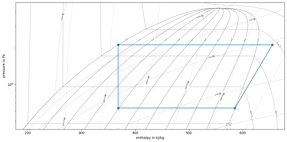
Alternatively we can use a library wrapping around CoolProp to plot styled diagrams, i.e. fluprodia.

from fluprodia import FluidPropertyDiagram
import numpy as np

fluid = "R290"
diagram = FluidPropertyDiagram(fluid)
diagram.set_unit_system(T="°C", h="kJ/kg")
diagram.set_isolines(T=np.arange(-25, 101, 25), s=np.arange(1250, 3001, 250), h=np.arange(100, 801, 100))
diagram.calc_isolines()

fig, ax = plt.subplots(1, figsize=(12, 6))

diagram.draw_isolines(fig, ax, "logph", _x_lims[0], _x_lims[1], _y_lims[0], _y_lims[1])
ax.scatter([h / 1e3 for h in [h_1, h_2, h_3, h_4]], [p_1, p_2, p_3, p_4])
ax.plot([h / 1e3 for h in [h_1, h_2, h_3, h_4, h_1]], [p_1, p_2, p_3, p_4, p_1])

ax.set_ylabel("pressure in Pa")
ax.set_xlabel("enthalpy in kJ/kg")

plt.tight_layout()

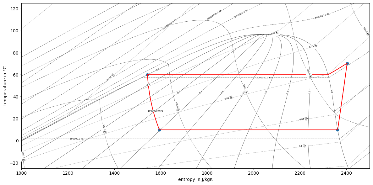
With this we can also easily put in a Ts diagram. To plot the lines, we have to follow the isobars, which are partly in the two-phase partly in overheated region. For this, fluprodia provides extra functionality.

fig, ax = plt.subplots(1, figsize=(12, 6))

diagram.draw_isolines(fig, ax, "Ts", 1000, 2500, -25, 125)

t = []
s = []
for p, h in zip([p_1, p_2, p_3, p_4], [h_1, h_2, h_3, h_4]):
    t += [PropsSI("T", "P", p, "H", h, fluid) - 273.15]
    s += [PropsSI("S", "P", p, "H", h, fluid)]

ax.scatter(s, t)

lines = {
    "12": {
        "isoline_property": "p",
        "isoline_value": p_1,
        "starting_point_property": "h",
        "starting_point_value": h_1 / 1e3,
        "ending_point_property": "h",
        "ending_point_value": h_2 / 1e3
    },
    "23": {
        "isoline_property": "s",
        "isoline_value": s[1],
        "isoline_value_end": s[2],
        "starting_point_property": "p",
        "starting_point_value": p_2,
        "ending_point_property": "p",
        "ending_point_value": p_3
    },
    "34": {
        "isoline_property": "p",
        "isoline_value": p_3,
        "starting_point_property": "h",
        "starting_point_value": h_3 / 1e3,
        "ending_point_property": "h",
        "ending_point_value": h_4 / 1e3
    },
    "41": {
        "isoline_property": "h",
        "isoline_value": h_4 / 1e3,
        "starting_point_property": "p",
        "starting_point_value": p_4,
        "ending_point_property": "p",
        "ending_point_value": p_1
    },
}

for line in lines.values():
    line_data = diagram.calc_individual_isoline(**line)
    ax.plot(line_data["s"], line_data["T"], color="#FF0000")

ax.set_ylabel("temperature in °C")
ax.set_xlabel("entropy in J/kgK")
plt.tight_layout()

Next we want to make a parametric study on the temperature level of evaporation and condensation. For that, we transform our small script to a function first.

def run_forward(fluid, t_2, t_4, eta_s, heat):
    p_2 = PropsSI("P", "T", t_2, "Q", 1, fluid)
    p_4 = PropsSI("P", "T", t_4, "Q", 0, fluid)

    h_2 = PropsSI("H", "T", t_2, "Q", 1, fluid)
    s_2 = PropsSI("S", "T", t_2, "Q", 1, fluid)

    p_3 = p_4
    h_3s = PropsSI("H", "S", s_2, "P", p_3, fluid)
    h_3 = h_2 + (h_3s - h_2) / eta_s

    h_4 = PropsSI("H", "T", t_4, "Q", 0, fluid)

    m = heat / (h_4 - h_3)
    power = m * (h_3 - h_2)
    cop = abs(heat) / power
    heat_evap = abs(heat) - power
    return m, power, cop, heat_evap

We can double-check, if we get the same result as previously:

fluid = "R290"
t_2 = 283.15
t_4 = 333.15
eta_s = 0.8
heat = -1e6

m, power, cop, heat_evap = run_forward(fluid, t_2, t_4, eta_s, heat)
round(cop, 2)

4.13

For the parametric study, we change both temperatures in a loop:

import pandas as pd


t_2_range = np.linspace(-15, 15, 31)
t_4_range = np.linspace(40, 70, 31)

cop_parametric = pd.DataFrame(index=t_2_range, columns=t_4_range)

for t_2 in t_2_range:
    _, _, cop, _ = run_forward(fluid, t_2 + 273.15, t_4_range + 273.15, eta_s, heat)
    cop_parametric.loc[t_2] = cop

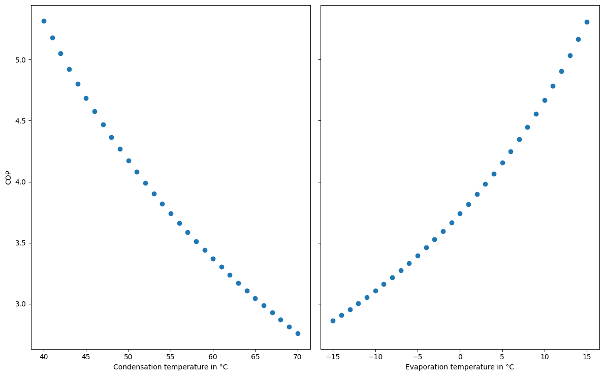
We can make two individual plots, which indicate the dependency of the COP, if we only change one or the other. As a base case, we select the middle temperature value on the ranges defined earlier.

fig, ax = plt.subplots(1, 2, sharey=True, figsize=(12, 7.5))

ax[0].scatter(cop_parametric.columns, cop_parametric.loc[0].values)
ax[0].set_xlabel("Condensation temperature in °C")
ax[0].set_ylabel("COP")
ax[1].scatter(cop_parametric.index, cop_parametric[55].values)
ax[1].set_xlabel("Evaporation temperature in °C")
plt.tight_layout()

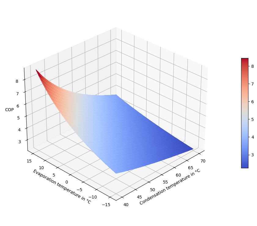
We can also make a 3D-surface plot using the temperature levels on x and y axes and the COP as z-value.

from matplotlib import cm

fig, ax = plt.subplots(1, figsize=(12, 7.5), subplot_kw={"projection": "3d"})

X, Y = np.meshgrid(t_4_range, t_2_range)

surf = ax.plot_surface(X, Y, cop_parametric.values, cmap=cm.coolwarm, linewidth=0, antialiased=False)

ax.set_xlabel("Condensation temperature in °C")
ax.set_ylabel("Evaporation temperature in °C")
ax.set_zlabel("COP")
ax.view_init(elev=30, azim=225)
ax.set_box_aspect(aspect=None, zoom=0.9)
fig.colorbar(surf, shrink=0.5, aspect=15)
plt.tight_layout()

Tasks part 2

The available compressor power is now limited to 200 kW.

• What amount of heat can the heat pump deliver in the conditions given in the table?

• What amount of heat can be delivered when the heat source temperature is reduced to 0 °C.

• At which heat source temperature level does the heat pump deliver 1 MW of heat again?

Reimplementation

For the first exercise we can reimplement our example straightforwardly: No temperature levels change, therefore only the calculation of the mass flow changes, i.e. via the compressor power and enthalpy difference instead of the condenser specifications.

fluid = "R290"
t_2 = 283.15
t_4 = 333.15
eta_s = 0.8
power = 200e3

p_2 = PropsSI("P", "T", t_2, "Q", 1, fluid)
p_4 = PropsSI("P", "T", t_4, "Q", 0, fluid)

h_2 = PropsSI("H", "T", t_2, "Q", 1, fluid)
s_2 = PropsSI("S", "T", t_2, "Q", 1, fluid)

p_3 = p_4
h_3s = PropsSI("H", "S", s_2, "P", p_3, fluid)
h_3 = h_2 + (h_3s - h_2) / eta_s

h_4 = PropsSI("H", "T", t_4, "Q", 0, fluid)
h_1 = h_4

m = power / (h_3 - h_2)
heat = m * (h_4 - h_3)
heat

-825429.7204056584

Similarly, we can reuse this implementation and simply change the value of \(T_2\).

t_2 = 273.15

p_2 = PropsSI("P", "T", t_2, "Q", 1, fluid)
p_4 = PropsSI("P", "T", t_4, "Q", 0, fluid)

h_2 = PropsSI("H", "T", t_2, "Q", 1, fluid)
s_2 = PropsSI("S", "T", t_2, "Q", 1, fluid)

p_3 = p_4
h_3s = PropsSI("H", "S", s_2, "P", p_3, fluid)
h_3 = h_2 + (h_3s - h_2) / eta_s

h_4 = PropsSI("H", "T", t_4, "Q", 0, fluid)
h_1 = h_4

m = power / (h_3 - h_2)
heat = m * (h_4 - h_3)
heat

-674011.0186535486

The third variant is a more complex: We want to have a power input of 200 kW and 1 MW of heat production at the same time and search for the temperature \(T_2\) to match that specification. Our only fixed point is the state number 4. The state 3 depends on the unknown state 2 via the isentropic efficiency equation:

\[h_3 = h(T=T_2, Q=1) + \frac{h\left(p=p_4, s=s\left(T=T_2, Q=1\right)\right) - h\left(T=T_2,Q=1\right)}{\eta_\text{cmp,s}}\]

Together with the specifications of the condenser heat production and compressor power input we would have to solve for \(T_2\) in this equation, which is not easily possible. Therefore, an iterative approach can be taken making use of our previous implementation.

Iterative calculations

We can implement a one-dimensional Newton algorithm to solve for the desired property. First, we can validate our implementation vs. the result we can from the first or second assignment.

power_new = 0.2e6
fluid = "R290"
power = 0
heat_guess = -1e6
t_2 = 283.15

d = 1e-6
while abs(power - power_new) > 1e-6:
    m, power, cop, heat_evap = run_forward(fluid, t_2, t_4, eta_s, heat_guess)
    residual = power - power_new
    heat_upper = heat_guess + d
    heat_lower = heat_guess - d
    _, power_upper, _, _ = run_forward(fluid, t_2, t_4, eta_s, heat_upper)
    _, power_lower, _, _ = run_forward(fluid, t_2, t_4, eta_s, heat_lower)
    derivative = (power_upper - power_lower) / (2 * d)
    heat_guess -= residual / derivative

heat_guess

-825429.7204056582

With the same strategy we can now update our temperature guess value and retrive it with both, power and heat, specified.

power_new = 0.2e6
fluid = "R290"
power = 0
heat = -1e6
d = 1e-6
t_2_guess = 333.15
while abs(power - power_new) > 1e-6:
    m, power, cop, heat_evap = run_forward(fluid, t_2_guess, t_4, eta_s, heat)
    residual = power - power_new
    t_2_upper = t_2_guess + d
    t_2_lower = t_2_guess - d
    _, power_upper, _, _ = run_forward(fluid, t_2_upper, t_4, eta_s, heat)
    _, power_lower, _, _ = run_forward(fluid, t_2_lower, t_4, eta_s, heat)
    derivative = (power_upper - power_lower) / (2 * d)
    t_2_guess -= residual / derivative

t_2_guess - 273.15

17.98695102553353