Exercises

Thermodynamic states and simple processes

1. Calculate the density and enthalpy of R290 at 5 bar and 50 °C.

2. What is the enthalpy of saturated liquid Ammonia at 75 °C.

3. Calculate the vapor mass fraction in the two-phase region of Ammonia at the same enthalpy but at a temperature of 25 °C.

4. At what temperature does Ammonia start to boil under a pressure of 4 bar.

5. What pressures correspond to a saturation temperature of 20 °C, 65 °C and 110 °C for water?

6. Calculate the entropy of R134a for the saturated vapor state at a temperature of 10 °C.

7. What is the temperature of R134a at the same entropy and twice as high pressure?

from CoolProp.CoolProp import PropsSI

PropsSI("D", "P", 5e5, "T", 50 + 273.15, "R290")

8.772185179043303

h = PropsSI("H", "Q", 0, "T", 75 + 273.15, "ammonia")
h

718053.520541121

p = PropsSI("P", "T", 25 + 273.15, "Q", 0, "ammonia")
PropsSI("Q", "H", h, "P", p, "ammonia")

0.21862680244396868

PropsSI("T", "P", 4e5, "Q", 0, "ammonia") - 273.15

-1.872698479668145

PropsSI("P", "T", [t + 273.15 for t in [20, 65, 110]], "Q", 0, "water")

array([  2339.31818827,  25041.59809182, 143378.71294487])

s = PropsSI("S", "T", 10 + 273.15, "Q", 1, "R134a")
p = PropsSI("P", "T", 10 + 273.15, "Q", 1, "R134a")
s

1722.111223569184

PropsSI("T", "S", s, "P", p * 2, "R134a") - 273.15

35.01696941125067

Refrigerants

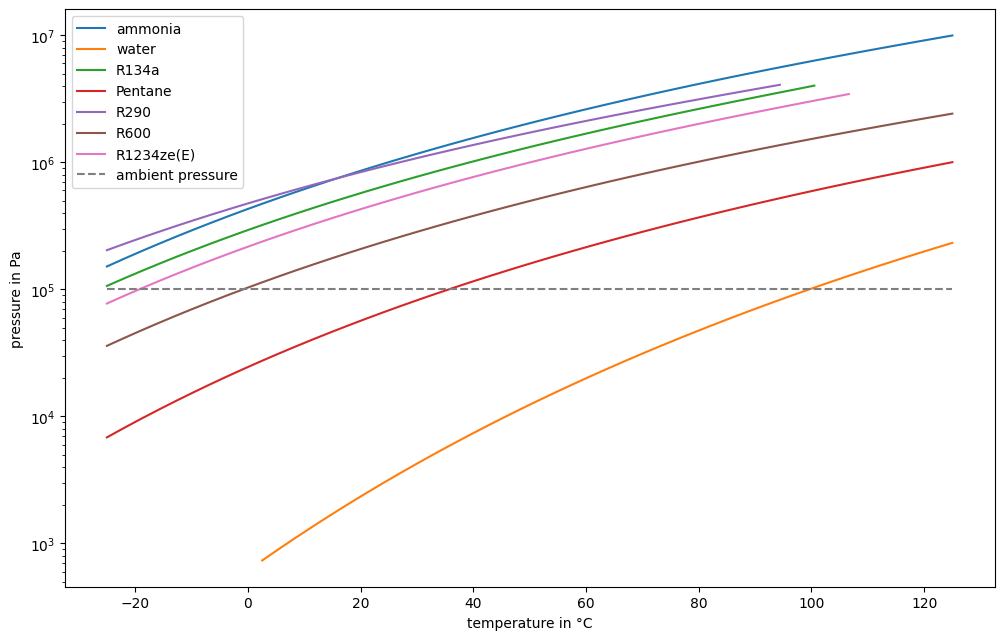
1. Plot the saturation curve for Ammonia, Water, R134a, R290, R600 and R1234ze(E) in a log-p,T diagram for temperature ranging from -25 °C to 125 °C.

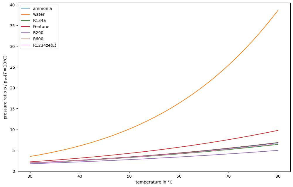
2. Plot the pressure ratio of saturation pressure vs. saturation pressure at 10 °C over a range of temperature values from 30 °C to 80 °C.

3. What factors may restrict the usage of the working fluids in heat pumps?

4. Calculate the entropy for the saturated liquid and vapor line same working fluids for temperature values larger than -25 °C. Plot the lines in a T-s diagram.

5. Compare the plots: What factors may restrict the usage of the working fluids in heat pumps?

from matplotlib import pyplot as plt
import numpy as np

fluids = ["ammonia", "water", "R134a", "Pentane", "R290", "R600", "R1234ze(E)"]
temperature = np.linspace(-25, 125)
saturation_pressure = {}
saturation_pressure_10 = {}
for fluid in fluids:
    saturation_pressure[fluid] = PropsSI("P", "T", temperature + 273.15, "Q", 0, fluid)
    saturation_pressure_10[fluid] = PropsSI("P", "T", 10 + 273.15, "Q", 0, fluid)

fig, ax = plt.subplots(1, figsize=(12, 7.5))

for fluid in fluids:
    ax.plot(temperature, saturation_pressure[fluid], label=fluid)

ax.set_yscale("log")
ax.set_ylabel("pressure in Pa")
ax.set_xlabel("temperature in °C")

ax.plot(temperature, [1e5] * len(temperature), "--", label="ambient pressure")
ax.legend()

<matplotlib.legend.Legend at 0x7f2054b4ef10>

temperature = np.linspace(30, 80)
saturation_pressure = {}
for fluid in fluids:
    saturation_pressure[fluid] = PropsSI("P", "T", temperature + 273.15, "Q", 0, fluid)

fig, ax = plt.subplots(1, figsize=(12, 7.5))

for fluid in fluids:
    ax.plot(temperature, saturation_pressure[fluid] / saturation_pressure_10[fluid], label=fluid)

ax.set_ylabel("pressure ratio")
ax.set_xlabel("temperature in °C")

ax.legend()

_ = ax.set_ylabel("pressure ratio p / p$_\\text{sat}\\left(T=10°C\\right)$")

• Operation below ambient pressure is challenging, since a vacuum has to be preserved. Therefore, for low temperature applications water, pentane and R600 are not very feasible.

• Similarly, very high pressure is requires a lot of technical effort. E.g. to reach 125 °C, Ammonia has to be compressed to about 100 bar.

• R290 and R134a have very good pressure ranges. R290 is explosive, R134a has a very high global warming potential (GWP), e.g. [6]

• Some reach critical point around 100 °C. In that region, the condensation section is small, therefore heat exchange has to happen with either larger surface area or higher temperature difference.

fig, ax = plt.subplots(1, figsize=(12, 8))

for fluid in fluids:
    temperature_range = np.linspace(-25 + 273.15, PropsSI("TCRIT", fluid))
    bubble_entropy = PropsSI("S", "T", temperature_range, "Q", 0, fluid)
    dew_entropy = PropsSI("S", "T", temperature_range, "Q", 1, fluid)
    _ = ax.plot(bubble_entropy, temperature_range - 273.15, label=fluid)
    color = _[0].get_color()
    ax.plot(dew_entropy, temperature_range - 273.15, color=color)

ax.set_ylabel("temperature in °C")
ax.set_xlabel("entropy in J/kgK")
_ = ax.legend()

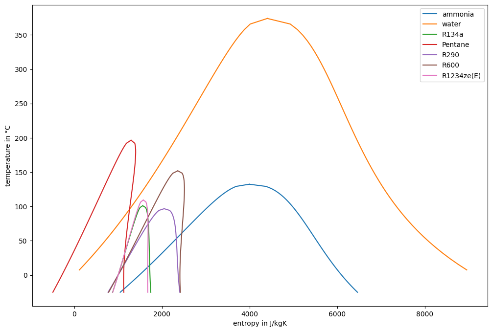
• Fluids can be categorized [7] (recently more detailed categories have been introduced [8]). The original categories were:

  • wet: dew line with negative slope (e.g. water, ammonia)

  • isentropic: dew line with infinite slope (e.g. R134a, R290, R1234ze(E))

  • dry: dew line with positive slope (e.g. Pentane, R600)

• Dry fluids (dewline leans over isentropics) risk compression into two-phase region, which may cause damage to the compressor.

• Small two-phase region indicates low heat of condensation (\(q=\int s dT\)) compared to desuperheating, which means higher heat exchange surface area required.

Component Models

Compressor

Implement a model, that allows you to model a compressor, where the compression process is adiabatic and reversible (isentropic).

1. What power does the compressor draw if 5 kg/s of R290 are compressed from saturated gaseous state at 15 °C to a pressure corresponding to a saturation temperature of 60 °C?

2. What is the outlet temperature?

3. How much mass can be compressed by the same machine, if 300 kW of power are available?

Now consider thermodynamic inefficiencies by incorporating isentropic efficiency in the model.

4. Assume isentropic efficiency of 80 %. What is the power, what is the outlet temperature?

5. The outlet temperature is measured to be 75 °C. What is the isentropic efficiency?

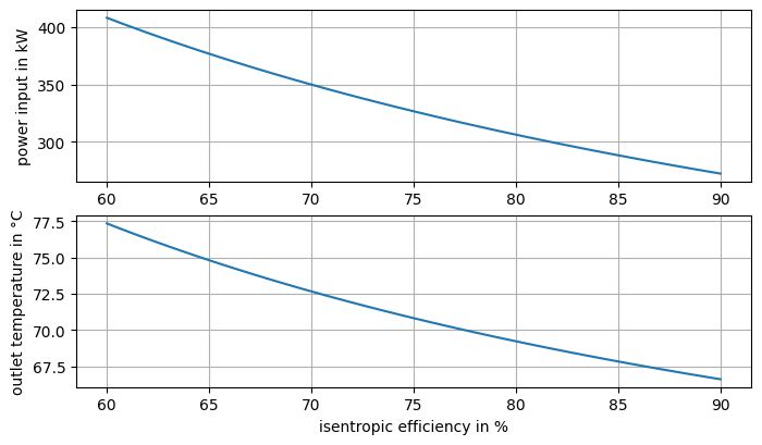
6. How does the compressor power requirement change as function of the isentropic efficiency with the starting point of the compression as in the first task. Plot the results.

We calculate the inlet and the outlet state of the compressor to determine the power. We index the outlet enthalpy in isentropic compression with an extra s.

\[\dot W = \dot m \cdot \left(h_\text{2,s} - h_1\right)\]

\[h_1 = h\left(T_1, Q\right)\]

\[h_\text{2,s} = h\left(p_2, s_1\right)\]

\[s_1 = s\left(T_1, Q\right)\]

\[p_2 = p_\text{sat}\left(T_\text{2,sat}\right)\]

fluid = "R290"
m = 5
t_1 = 15 + 273.15
t_2sat = 60 + 273.15

p_1 = PropsSI("P", "T", t_1, "Q", 1, fluid)

h_1 = PropsSI("H", "P", p_1, "Q", 1, fluid)
s_1 = PropsSI("S", "P", p_1, "Q", 1, fluid)

p_2 = PropsSI("P", "T", t_2sat, "Q", 1, fluid)
h_2s = PropsSI("H", "S", s_1, "P", p_2, fluid)

power = m * (h_2s - h_1)
power

245022.95536683116

Outlet temperature can be determined from the outlet pressure and the outlet enthalpy.

t_2s = PropsSI("T", "H", h_2s, "P", p_2, fluid)
t_2s - 273.15

64.55082012287357

With a different power output and the same inlet conditions and compressor efficiency only the mass flow changes.

\[\dot m = \frac{\dot W}{h_\text{2,s} - h_1}\]

power = 300e3
m = power / (h_2s - h_1)
m

6.121875388182733

With compressor efficiency we can calculate the actual outlet enthalpy based on the outlet enthalpy in isentropic condition (\(h_2\) in the previous section).

\[h_2 = h_1 + \frac{h_\text{2,s} - h_1}{\eta_\text{s}}\]

eta_s = 0.8
m = 5
h_2 = h_1 + (h_2s - h_1) / eta_s
power = m * (h_2 - h_1)
power

306278.6942085391

As previously we can calculate the outlet temperature.

PropsSI("T", "H", h_2, "P", p_2, fluid) - 273.15

69.22446442457743

If the outlet temperature is an input, the isentropic efficiency can be calculated by first determining the outlet enthalpy.

\[h_2 = h\left(T_2, p_2\right)\]

\[\eta_\text{s} = \frac{h_\text{2,s} - h_1}{h_2 - h_1}\]

t_2 = 75
h_2 = PropsSI("H", "T", t_2 + 273.15, "P", p_2, fluid)
(h_2s - h_1) / (h_2 - h_1)

0.6461310700391392

We can vary the efficiency over a range and then calculate the corresponding outlet enthalpy, temperature and power value and then make a plot of the curves.

import numpy as np

eta_s_range = np.linspace(0.6, 0.9)
h_2_range = h_1 + (h_2s - h_1) / eta_s_range
t_2_range = PropsSI("T", "P", p_2, "H", h_2_range, fluid)
power_range = m * (h_2_range - h_1)

fig, ax = plt.subplots(2, figsize=(8, 4.5))

eta_s_range *= 100
power_range /= 1e3
t_2_range -= 273.15

ax[0].plot(eta_s_range, power_range)
ax[0].set_ylabel("power input in kW")
ax[1].plot(eta_s_range, t_2_range)
ax[1].set_ylabel("outlet temperature in °C")
ax[1].set_xlabel("isentropic efficiency in %")

ax[0].grid()
ax[1].grid()

Heat exchanger

1. How much heat is required to completely evaporate 3 kg/s saturated liquid R134a at 10, 20 and 30 °C?

2. Which volumetric flow of air is required to provide the heat in any of the three cases? Assume, that the minimal temperature difference between the air and the working fluid is 3 °C and the air temperature changes by 5 °C.

3. Which volumetric flow of water is required under the same circumstances?

4. What information can you transfer to the heat exchanger design?

The heat can be obtained from the change of state similar to before:

\[\dot Q = \dot m \cdot \left(h_2 - h_1\right)\]

\[h_1 = h\left(T_\text{sat},Q=0\right)\]

\[h_2 = h\left(T_\text{sat},Q=1\right)\]

m = 3
working_fluid = "R134a"
t = [_t + 273.15 for _t in [10, 20, 30]]
h_1 = PropsSI("H", "T", t, "Q", 0, working_fluid)
h_2 = PropsSI("H", "T", t, "Q", 1, working_fluid)

heat = m * (h_2 - h_1)
heat

array([572222.64320289, 546841.76912514, 519288.35855779])

First we calculate the mass flow of air required to be heated up by 5 K when the heat is transferred from the working fluid evaporation.

\[\dot m_\text{air} = \frac{-\dot Q}{h_\text{air,2} - h_\text{air,1}}\]

\[h_\text{air} = h\left(p,T\right)\]

\[T_\text{air,2} = T_\text{wf} + 3 K\]

\[T_\text{air,1} = T_\text{air,2} - 5\]

t_source_2 = np.array(t) + 3
t_source_1 = t_source_2 + 5
p_source = 1e5
fluid = "air"

h_source_1 = PropsSI("H", "T", t_source_1, "P", p_source, fluid)
h_source_2 = PropsSI("H", "T", t_source_2, "P", p_source, fluid)

m_source = -heat / (h_source_2 - h_source_1)
m_source

array([113.76295821, 108.68306959, 103.16654506])

We can use the inlet specific volume to calculate the volumetric flow based on the mass flow.

\[v = \frac{1}{\rho}\]

\[\rho = \rho\left(p,T\right)\]

v_source_1 = 1 / PropsSI("D", "T", t_source_1, "P", p_source, fluid)
m_source * v_source_1

array([95.03949204, 93.92287791, 92.1234932 ])

We can do the same with water instead of air on the heat source side.

fluid = "water"

h_source_1 = PropsSI("H", "T", t_source_1, "P", p_source, fluid)
h_source_2 = PropsSI("H", "T", t_source_2, "P", p_source, fluid)

m_source = -heat / (h_source_2 - h_source_1)
m_source

array([27.32661279, 26.15736131, 24.8506327 ])

v_source_1 = 1 / PropsSI("D", "T", t_source_1, "P", p_source, fluid)
m_source * v_source_1

array([0.02736498, 0.02625621, 0.02502668])

• High volumetric flow means either high flow speed or very large heat exchange area.

• Pressure losses are extra costly with high volumetric flow, blowers/fans draw a lot of power.

• Water has higher density and also higher mass specific heat capacity. Change of temperature is lower for any given flowrate.