Heat Pump

Introduction

Fig. 20 Flow sheet of the simplest implementation of a heat pump.

As the final simple thermodynamic cycle, a heat pump will be subject of the exergy analysis. Heat pumps are a promising technology in the process of climate change mitigation, because they can replace conventional fossil fuel based heating plants. As heat pumps are scalable, they can be used in households and building, as well as whole neighbourhoods and in district heating systems. A heat pump employs the well known refrigeration cycle (see Fig. 20), but instead uses the heat that is transferred out of the system. For the cycle to work, heat has to be transferred into the system at a lower temperature level and through the input of work can be transferred out on a higher temperature level. The resulting energy balance of a heat pump is displayed in Eq. (41).

(41)\[ 0 = Q_{in} + Q_{out} + W_{in}\]

As traditionally is done with heat engines, the benefit of a cycle can be put in to relation with the necessary input. Formalizing this expression yields the so-called coefficient of performance of a heat pump, as is shown in Eq. (42). From the energy balance (41) we can infer, that the outgoing heat is the sum of the work and heat put in. This means, that the \(COP\) must be greater than \(1\), in contrast to the thermal efficiency of heat engines.

(42)\[ COP = \frac{Q_{out}}{W_{in}}\]

Coming from thermal efficiencies of heat engines, this can seem to be in conflict the laws of thermodynamics. We get more heat from the cycle than work needs to be put in. There only has to be an ambient heat source supply heat at a lower temperature. To reveal the thermodynamic losses occurring in this process and to show that the cycle is no perpetuum mobile, we can analyze the exergy flows.

At first, we have to define the fuel and the product of the heat pump cycle. As described above, the benefit of the cycle is the heat transferred out of the system, which makes it the product. The necessary fuels logically are the heat and work inputs. Added to the compressor work are necessary supplemental work inputs like recirculation pumps. With these defined, we can start to build the heat pump model.

Exercise 1

1. Build a simple heat pump model using ammonia with TESPy according to the flowsheet in Fig. 20, but add a water fed heat source (the hot side of the evaporator) and a consumer cycle as the heat sink (the cold side of the condenser). Parametrize the model according to the description as shown in Table 4.

2. Execute the exergy analysis for the heat pump model. Visualize how each component destroys part of the fuel exergy through a waterfall diagram. Analyze the influence of the compressors isentropic efficiency, as well as that of the heat exchangers terminal temperature differences.

3. Analyze the impact of the ambient temperature level on the components and total efficiency.

Table 4 Parametrization of the heat pump

Description	Parameter	Value	Unit
Compressor	Isentropic efficiency	75	%
	Motor efficiency	96	%
Pumps	Isentropic efficiency	80	%
	Motor efficiency	96	%
All Heat Exchangers	Pressure losses	2	%
	Terminal temperature difference	2	K
Heat Sink	Nominal heat demand	-500	kW
	Feed flow temperature	70	°C
	Back flow temperature	50	°C
	System pressure	10	bar
Heat Source	Incoming temperature	10	°C
	Temperature reduction	5	K
	System pressure	1.013	bar

Note

If you are heaving trouble with the simulation not converging, try setting best guesses for pressures instead of terminal temperature differences and only after a succesful simulation reset the intended values (see also the TESPy tutorial on How to Generate Stable Starting Values).

Note

If you are encountering problems with specific components during the exergy analysis, try having a look at the individual components API documentation and their respective implementation of the exergy_balance method.

Proposed solution 1.1

First step: Build the heat pump model topology

Show code cell content Hide code cell content

from tespy.networks import Network
from tespy.connections import Connection, Bus
from tespy.components import (
    CycleCloser, Source, Sink, Pump, HeatExchanger, Condenser,
    HeatExchangerSimple, Compressor, Valve
    )

# Network
refrigerant = 'Ammonia'
nw = Network(
    fluids=[refrigerant, 'water'],
    T_unit='C', p_unit='bar', h_unit='kJ / kg', m_unit='kg / s'
)

# Components
cycle_closer = CycleCloser('Refrigerant Cycle Closer')

heatsource_ff = Source('Heat Source Feed Flow')
evaporator = HeatExchanger('Evaporator')
heatsource_pump = Pump('Heat Source Recirculation Pump')
heatsource_bf = Sink('Heat Source Back Flow')

compressor = Compressor('Compressor')

cons_cc = CycleCloser('Consumer Cycle Closer')
cons_pump = Pump('Heat Sink Recirculation Pump')
condenser = Condenser('Condenser')
cons_heatsink = HeatExchangerSimple('Heat Consumer')

valve = Valve('Expansion Valve')

# Connections
cond2cc = Connection(condenser, 'out1', cycle_closer, 'in1', label='00')
cc2valve = Connection(cycle_closer, 'out1', valve, 'in1', label='01')
valve2eva = Connection(valve, 'out1', evaporator, 'in2', label='02')

nw.add_conns(cond2cc, cc2valve, valve2eva)

hs_ff2evap = Connection(heatsource_ff, 'out1', evaporator, 'in1', label='21')
evap2hs_pump = Connection(evaporator, 'out1', heatsource_pump, 'in1', label='22')
hs_pump2hs_bf = Connection(heatsource_pump, 'out1', heatsource_bf, 'in1', label='23')

nw.add_conns(hs_ff2evap, evap2hs_pump, hs_pump2hs_bf)

evap2comp = Connection(evaporator, 'out2', compressor, 'in1', label='03')
comp2cond = Connection(compressor, 'out1', condenser, 'in1', label='04')

nw.add_conns(evap2comp, comp2cond)

cons_cc2cons_pump = Connection(cons_cc, 'out1', cons_pump, 'in1', label='30')
cons_pump2cond = Connection(cons_pump, 'out1', condenser, 'in2', label='31')
cond2cons_hs = Connection(condenser, 'out2', cons_heatsink, 'in1', label='32')
cons_hs2cons_cc = Connection(cons_heatsink, 'out1', cons_cc, 'in1', label='33')

nw.add_conns(cons_cc2cons_pump, cons_pump2cond, cond2cons_hs, cons_hs2cons_cc)

Second step: Set the heat pumps process parameters and starting values. After that define the energy busses and solve model with starting and final values.

Show code cell content Hide code cell content

from CoolProp.CoolProp import PropsSI as PSI
from tespy.tools import ExergyAnalysis

# Component parameters
compressor.set_attr(eta_s=0.75)
cons_pump.set_attr(eta_s=0.8)
heatsource_pump.set_attr(eta_s=0.8)

evaporator.set_attr(pr1=0.98, pr2=0.98)
condenser.set_attr(pr1=0.98, pr2=0.98)
cons_heatsink.set_attr(pr=0.98, Q=-500e3, dissipative=False)

# Connection parameters
cond2cons_hs.set_attr(T=70, p=10, fluid={refrigerant: 0, 'water': 1})
cons_hs2cons_cc.set_attr(T=50)

hs_ff2evap.set_attr(T=10, p=1.013, fluid={refrigerant: 0, 'water': 1})
evap2hs_pump.set_attr(T=5)
hs_pump2hs_bf.set_attr(p=1.013)

evap2comp.set_attr(x=1, fluid={refrigerant: 1, 'water': 0})

# Starting values
p_evap = PSI('P', 'Q', 1, 'T', 5 - 2 + 273.15, refrigerant)
evap2comp.set_attr(p=p_evap*1e-5)

p_cond = PSI('P', 'Q', 0, 'T', 70 + 2 + 273.15, refrigerant)
cond2cc.set_attr(p=p_cond*1e-5)

# Busses
heat_in = Bus('Heat Input')
heat_in.add_comps(
    {'comp': heatsource_ff, 'base': 'bus'},
    {'comp': heatsource_bf, 'base': 'component'}
    )

heat_out = Bus('Heat Output')
heat_out.add_comps(
    {'comp': cons_heatsink, 'base': 'component'})

power_in = Bus('Power Input')
power_in.add_comps(
    {'comp': compressor, 'char': 0.96, 'base': 'bus'},
    {'comp': heatsource_pump, 'char': 0.96, 'base': 'bus'},
    {'comp': cons_pump, 'char': 0.96, 'base': 'bus'}
    )

nw.add_busses(heat_in, heat_out, power_in)

# Initial solve with starting values
nw.set_attr(iterinfo=False)
nw.solve('design')

# Final solve 
evap2comp.set_attr(p=None)
evaporator.set_attr(ttd_l=2)

cond2cc.set_attr(p=None)
condenser.set_attr(ttd_u=2)

nw.solve('design')
print(f'COP = {abs(heat_out.P.val)/power_in.P.val:.3f}')

COP = 3.060

Proposed solution 1.2

First step: Create and execute ExergyAnalysis instance

Show code cell content Hide code cell content

from tespy.tools import ExergyAnalysis

ean = ExergyAnalysis(network=nw, E_F=[heat_in, power_in], E_P=[heat_out])
ean.analyse(pamb=1.013, Tamb=25)
ean.print_results(groups=False, connections=False, components=False, busses=False)

##### RESULTS: Aggregation of components and busses #####
+--------------------------------+-------------+-------------+-------------+-------------+-------------+-------------+
|                                |         E_F |         E_P |         E_D |     epsilon |        y_Dk |       y*_Dk |
|--------------------------------+-------------+-------------+-------------+-------------+-------------+-------------|
| Condenser                      |   8.577e+04 |   5.238e+04 |   3.339e+04 |   6.107e-01 |   2.351e-01 |   3.725e-01 |
| Compressor                     |   1.640e+05 |   1.316e+05 |   3.237e+04 |   8.025e-01 |   2.279e-01 |   3.612e-01 |
| Expansion Valve                |   4.488e+04 |   2.820e+04 |   1.668e+04 |   6.284e-01 |   1.174e-01 |   1.861e-01 |
| Evaporator                     |   2.840e+04 |   2.141e+04 |   6.989e+03 |   7.539e-01 |   4.921e-02 |   7.798e-02 |
| Heat Consumer                  |   5.251e+04 |   5.239e+04 |   1.198e+02 |   9.977e-01 |   8.436e-04 |   1.337e-03 |
| Heat Sink Recirculation Pump   |   3.181e+02 |   2.490e+02 |   6.906e+01 |   7.829e-01 |   4.863e-04 |   7.706e-04 |
| Heat Source Recirculation Pump |   4.380e+01 |   3.320e+01 |   1.060e+01 |   7.581e-01 |   7.461e-05 |   1.182e-04 |
| Refrigerant Cycle Closer       | nan         | nan         | nan         | nan         | nan         | nan         |
| Heat Source Feed Flow          | nan         | nan         | nan         | nan         | nan         | nan         |
| Heat Source Back Flow          | nan         | nan         | nan         | nan         | nan         | nan         |
| Consumer Cycle Closer          | nan         | nan         | nan         | nan         | nan         | nan         |
+--------------------------------+-------------+-------------+-------------+-------------+-------------+-------------+
##### RESULTS: Network exergy analysis #####
+-----------+-----------+-----------+-----------+-----------+
|       E_F |       E_P |       E_D |       E_L |   epsilon |
|-----------+-----------+-----------+-----------+-----------|
| 1.420e+05 | 5.239e+04 | 8.963e+04 | 0.000e+00 | 3.689e-01 |
+-----------+-----------+-----------+-----------+-----------+

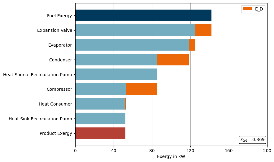
Second step: Prepare data and plot waterfall diagram of the heat pump process

Show code cell content Hide code cell content

import matplotlib.pyplot as plt
import numpy as np

comps = ['Fuel Exergy']
E_F = ean.network_data.E_F
E_D = [0]
E_P = [E_F]
for comp in ean.aggregation_data.index:
    # only plot components with exergy destruction > 1 W
    if ean.aggregation_data.E_D[comp] > 1 :
        comps.append(comp)
        E_D.append(ean.aggregation_data.E_D[comp])
        E_F = E_F - ean.aggregation_data.E_D[comp]
        E_P.append(E_F)
comps.append('Product Exergy')
E_D.append(0)
E_P.append(E_F)

E_D = [E * 1e-3 for E in E_D]
E_P = [E * 1e-3 for E in E_P]

colors_E_P = ['#74ADC0'] * len(comps)
colors_E_P[0] = '#00395B'
colors_E_P[-1] = '#B54036'

fig, ax = plt.subplots(figsize=(8, 6))

ax.barh(np.arange(len(comps)), E_P, align='center', color=colors_E_P)
ax.barh(np.arange(len(comps)), E_D, align='center', left=E_P, label='E_D', color='#EC6707')

ax.legend()
ax.annotate(
    f'$\epsilon_{{tot}} = ${ean.network_data["epsilon"]:.3f}', (0.86, 0.04),
    xycoords='axes fraction',
    ha='left', va='center', color='k',
    bbox=dict(boxstyle='round,pad=0.3', fc='white')
    )
ax.set_xlabel('Exergy in kW')
ax.set_yticks(np.arange(len(comps)))
ax.set_yticklabels(comps)
ax.set_xlim([0, 200])
ax.set_xticks(np.linspace(0, 200, 6))
ax.invert_yaxis()
ax.grid(axis='x')
ax.set_axisbelow(True)

Third step: Variate compressor isentropic efficiency and terminal temperature differences of evaporator and condenser

Show code cell content Hide code cell content

def get_ean_results(ean, comps):
    E_F = ean.network_data.E_F * 1e-3
    E_D = [0]
    E_P = [E_F]

    for comp in comps[1:-1]:
        E_D += [ean.aggregation_data.E_D[comp] * 1e-3]
        E_F -= E_D[-1]
        E_P += [E_F]

    E_D += [0]
    E_P += [E_F]

    return E_P, E_D

eta_s_range = np.linspace(0.65, 0.8, 4)
ttd_range = np.arange(2, 10, 2)
comps = [
    'Fuel Exergy', 'Expansion Valve', 'Evaporator', 'Compressor', 'Condenser',
    'Product Exergy'
    ]

fig, axs = plt.subplots(
    len(ttd_range), len(eta_s_range),
    sharex=True, sharey=True, figsize=(14, 14)
    )
axs[0, 0].invert_yaxis()

for col, eta_s in enumerate(eta_s_range):
    compressor.set_attr(eta_s=eta_s)
    for row, ttd in enumerate(ttd_range):
        evaporator.set_attr(ttd_l=ttd)
        condenser.set_attr(ttd_u=ttd)

        nw.solve('design')
        ean = ExergyAnalysis(network=nw, E_F=[heat_in, power_in], E_P=[heat_out])
        ean.analyse(pamb=1.013, Tamb=25)

        E_P, E_D = get_ean_results(ean, comps)

        colors_E_P = ['#74ADC0'] * len(comps)
        colors_E_P[0] = '#00395B'
        colors_E_P[-1] = '#B54036'

        axs[row, col].barh(
            np.arange(len(comps)), E_P, align='center', color=colors_E_P
            )
        axs[row, col].barh(
            np.arange(len(comps)), E_D, align='center', left=E_P, label='E_D', color='#EC6707'
            )

        axs[row, col].set_yticks(np.arange(len(comps)))
        axs[row, col].set_yticklabels(comps)
        axs[row, col].grid(axis='x')
        axs[row, col].set_axisbelow(True)
        axs[row, col].set_xlim([0, 200])
        axs[row, col].set_xticks(np.linspace(0, 200, 5))

        axs[row, col].annotate(
                    f'$\epsilon_{{tot}} = ${ean.network_data["epsilon"]:.3f}', (0.635, 0.07),
                    xycoords='axes fraction',
                    ha='left', va='center', color='k',
                    bbox=dict(boxstyle='round,pad=0.3', fc='white')
                    )

        if row == len(ttd_range)-1:
            axs[row, col].set_xlabel(f'Isentropic Efficiency {eta_s:.2f}')
        if col == 0:
            axs[row, col].set_ylabel(f'Terminal temperature difference {ttd} K')

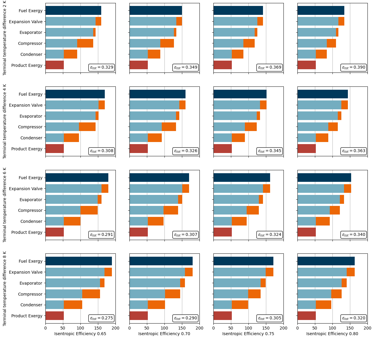
Explanation

Bei konstanten Umgebungs, Quellen- und Senkentemperaturen:

• Wenn ttd_u am Cond steigt, steigt die Kondensationstemperatur –> höhere Destruction im Cond am Comp –> höheres Fuel Exergy und schlechteres epsilon

• Wenn ttd_l am Evap steigt, sinkt die Verdampfungstemperatur weiter unter T_0 –> höhere Destruction im Evap und Valve –> höheres Fuel Exergy und schlechteres epsilon

• Wenn eta_s am Comp steigt, sinkt die Verdichteraustrittstemperatur –> niedigere Destruction im Comp und Cond –> geringeres Fuel Exergy und besseres epsilon

Proposed solution 1.3

First step: Variate ambient temperature and analyze the effect on total efficiency.

Show code cell content Hide code cell content

# Reset the isentropic efficiency and terminal temperature differences
compressor.set_attr(eta_s=0.75)
evaporator.set_attr(ttd_l=2)
condenser.set_attr(ttd_u=2)
nw.solve('design')

T_amb_range = np.linspace(5, 35, 4)
comps = [
    'Fuel Exergy', 'Expansion Valve', 'Evaporator', 'Compressor', 'Condenser',
    'Product Exergy'
    ]

fig, axs = plt.subplots(len(T_amb_range), 1, sharex=True, sharey=True, figsize=(8, 14))
axs[0].invert_yaxis()

for row, T_amb in enumerate(T_amb_range):
    ean = ExergyAnalysis(network=nw, E_F=[heat_in, power_in], E_P=[heat_out])
    ean.analyse(pamb=1.013, Tamb=T_amb)

    E_P, E_D = get_ean_results(ean, comps)

    colors_E_P = ['#74ADC0'] * len(comps)
    colors_E_P[0] = '#00395B'
    colors_E_P[-1] = '#B54036'

    axs[row].barh(
        np.arange(len(comps)), E_P, align='center', color=colors_E_P
        )
    axs[row].barh(
        np.arange(len(comps)), E_D, align='center', left=E_P, label='E_D', color='#EC6707'
        )

    axs[row].set_yticks(np.arange(len(comps)))
    axs[row].set_yticklabels(comps)
    axs[row].grid(axis='x')
    axs[row].set_axisbelow(True)
    axs[row].set_xlim([0, 200])
    axs[row].set_xticks(np.linspace(0, 200, 6))

    axs[row].annotate(
                f'$\epsilon_{{tot}} = ${ean.network_data["epsilon"]:.3f}', (0.86, 0.075),
                xycoords='axes fraction',
                ha='left', va='center', color='k',
                bbox=dict(boxstyle='round,pad=0.3', fc='white')
                )
    axs[row].set_ylabel(f'Ambient temperature {T_amb} K')

axs[row].set_xlabel('Exergy in kW')

Text(0.5, 0, 'Exergy in kW')

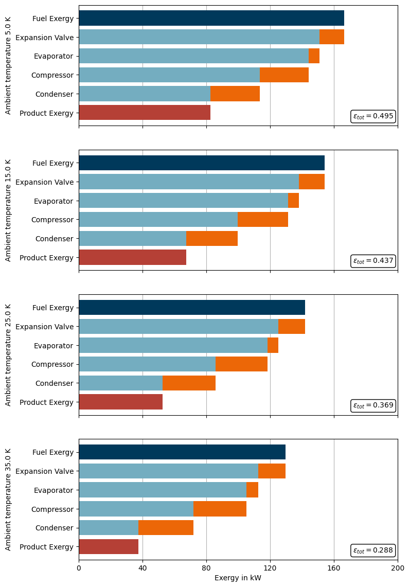
Second step: Analyze the exergy effect on the components and compare it at different ambient temperatures.

Comparison of energy and exergy efficiency

Table 5 Comparison of exergy efficiencies of each components at different ambient temperatures

	5°C	15°C	25°C	35°C
Expansion Valve	13.8 %	48.5 %	62.8 %	82.3 %
Evaporator	0 %	57.6 %	75.4 %	70.7 %
Compressor	81.2 %	80.7 %	80.3 %	79.8 %
Condenser	72.6 %	67.6 %	61.1 %	52.0 %
Total Network	49.5 %	43.7 %	36.9 %	28.8 %

Explanation

Hier könnte ihre Erklärung stehen

Topological process improvements

There are many ways to improve a heat pumps \(COP\) by changing the process through the addition of components. A popular topological improvement is the so-called Economizer, where part of the condensate gets evaporated on an intermediate pressure level and injected between two compressor stages. This is done in order to yield a cooler mixture entering the high pressure compressor and to reduce the final output temperature of the superheated gas. The evaporation of part of the condensate is reached through subcooling of the rest of it via an internal heat exchanger. The topology of this improved heat pump cycle can be seen in the flowsheet depicted in Fig. 21.

Fig. 21 Flow sheet of a heat pump with an economizer.

Exercise 2

Build the heat pump model including the economizer according to the flowsheet (see Fig. 21) and the parametrization of Table 4. Additionally, you need to set the distribution of the mass flow at the splitter, as well as the intermediate pressure at the economizer. Explain the improvement of the heat pumps \(COP\) by analyzing the exergy destruction of each component.

Proposed solution 2

First step: Build the extenden heat pump cycle with economizer

Show code cell content Hide code cell content

from tespy.connections import Ref
from tespy.components import Merge, Splitter

# Network
refrigerant = 'Ammonia'
nw_econ = Network(
    fluids=[refrigerant, 'water'],
    T_unit='C', p_unit='bar', h_unit='kJ / kg', m_unit='kg / s'
)

# Components
cycle_closer = CycleCloser('Refrigerant Cycle Closer')
split = Splitter('Condensate Splitter')
economizer = HeatExchanger('Economizer')
valve = Valve('Main Valve')
intermediate_valve = Valve('Intermediate Valve')

heatsource_ff = Source('Heat Source Feed Flow')
evaporator = HeatExchanger('Evaporator')
heatsource_pump = Pump('Heat Source Recirculation Pump')
heatsource_bf = Sink('Heat Source Back Flow')

lp_compressor = Compressor('Low Pressure Compressor')
merge = Merge('Injection')
hp_compressor = Compressor('High Pressure Compressor')

cons_cc = CycleCloser('Consumer Cycle Closer')
cons_pump = Pump('Heat Sink Recirculation Pump')
condenser = Condenser('Condenser')
cons_heatsink = HeatExchangerSimple('Heat Consumer')

# Connections
cond2cc = Connection(condenser, 'out1', cycle_closer, 'in1', label='00')
cc2split = Connection(cycle_closer, 'out1', split, 'in1', label='01')
split2econ = Connection(split, 'out1', economizer, 'in1', label='02')
econ2main_valve = Connection(economizer, 'out1', valve, 'in1', label='03')
main_valve2evap = Connection(valve, 'out1', evaporator, 'in2', label='04')

nw_econ.add_conns(cond2cc, cc2split, split2econ, econ2main_valve, main_valve2evap)

hs_ff2evap = Connection(heatsource_ff, 'out1', evaporator, 'in1', label='21')
evap2hs_pump = Connection(evaporator, 'out1', heatsource_pump, 'in1', label='22')
hs_pump2hs_bf = Connection(heatsource_pump, 'out1', heatsource_bf, 'in1', label='23')

nw_econ.add_conns(hs_ff2evap, evap2hs_pump, hs_pump2hs_bf)

evap2lp_comp = Connection(evaporator, 'out2', lp_compressor, 'in1', label='05')
lp_comp2merge = Connection(lp_compressor, 'out1', merge, 'in1', label='06')
merge2hp_comp = Connection(merge, 'out1', hp_compressor, 'in1', label='07')
hp_comp2cond = Connection(hp_compressor, 'out1', condenser, 'in1', label='08')

nw_econ.add_conns(evap2lp_comp, lp_comp2merge, merge2hp_comp, hp_comp2cond)

cons_cc2cons_pump = Connection(cons_cc, 'out1', cons_pump, 'in1', label='30')
cons_pump2cond = Connection(cons_pump, 'out1', condenser, 'in2', label='31')
cond2cons_hs = Connection(condenser, 'out2', cons_heatsink, 'in1', label='32')
cons_hs2cons_cc = Connection(cons_heatsink, 'out1', cons_cc, 'in1', label='33')

nw_econ.add_conns(cons_cc2cons_pump, cons_pump2cond, cond2cons_hs, cons_hs2cons_cc)

split2inter_valve = Connection(split, 'out2', intermediate_valve, 'in1', label='09')
inter_valve2econ = Connection(intermediate_valve, 'out1', economizer, 'in2', label='10')
econ2merge = Connection(economizer, 'out2', merge, 'in2', label='11')

nw_econ.add_conns(split2inter_valve, inter_valve2econ, econ2merge)

# Component parameters
lp_compressor.set_attr(eta_s=0.75)
hp_compressor.set_attr(eta_s=0.75)
cons_pump.set_attr(eta_s=0.8)
heatsource_pump.set_attr(eta_s=0.8)

evaporator.set_attr(pr1=0.98, pr2=0.98)
condenser.set_attr(pr1=0.98, pr2=0.98)
economizer.set_attr(pr1=0.98, pr2=0.98)
cons_heatsink.set_attr(pr=0.98, Q=-500e3, dissipative=False)

# Connection parameters
cond2cons_hs.set_attr(T=70, p=10, fluid={refrigerant: 0, 'water': 1})
cons_hs2cons_cc.set_attr(T=50)

hs_ff2evap.set_attr(T=10, p=1.013, fluid={refrigerant: 0, 'water': 1})
evap2hs_pump.set_attr(T=5)
hs_pump2hs_bf.set_attr(p=1.013)

evap2lp_comp.set_attr(x=1)
cond2cc.set_attr(fluid={refrigerant: 1, 'water': 0})

split2econ.set_attr(m=Ref(hp_comp2cond, 0.85, 0))

# Starting values
p_evap = PSI('P', 'Q', 1, 'T', 5 - 2 + 273.15, refrigerant) * 1e-5
main_valve2evap.set_attr(p=p_evap)
p_cond = PSI('P', 'Q', 0, 'T', 70 + 2 + 273.15, refrigerant) * 1e-5
hp_comp2cond.set_attr(p=p_cond)
p_mid = np.sqrt(p_evap * p_cond)
econ2merge.set_attr(p=p_mid, x=1)

# Busses
heat_in = Bus('Heat Input')
heat_in.add_comps(
    {'comp': heatsource_ff, 'base': 'bus'},
    {'comp': heatsource_bf, 'base': 'component'}
    )

heat_out = Bus('Heat Output')
heat_out.add_comps(
    {'comp': cons_heatsink, 'base': 'component'})

power_in = Bus('Power Input')
power_in.add_comps(
    {'comp': lp_compressor, 'char': 0.96, 'base': 'bus'},
    {'comp': hp_compressor, 'char': 0.96, 'base': 'bus'},
    {'comp': heatsource_pump, 'char': 0.96, 'base': 'bus'},
    {'comp': cons_pump, 'char': 0.96, 'base': 'bus'}
    )

nw_econ.add_busses(heat_in, heat_out, power_in)

# Initial solve with starting values
nw_econ.set_attr(iterinfo=False)
nw_econ.solve('design')

# Final solve 
main_valve2evap.set_attr(p=None)
evaporator.set_attr(ttd_l=2)
hp_comp2cond.set_attr(p=None)
condenser.set_attr(ttd_u=2)

nw_econ.solve('design')

print(f'COP = {abs(heat_out.P.val)/power_in.P.val:.3f}')

COP = 3.178

Second step: Create and execute ExergyAnalysis instance and plot the waterfall diagram of the heat pump with economizer

Show code cell content Hide code cell content

ean_econ = ExergyAnalysis(network=nw_econ, E_F=[heat_in, power_in], E_P=[heat_out])
ean_econ.analyse(pamb=1.013, Tamb=25)
ean_econ.print_results(groups=False, connections=False, components=False, busses=False)

comps = [
    'Fuel Exergy', 'Economizer', 'Main Valve', 'Evaporator', 'Low Pressure Compressor', 
    'Injection', 'High Pressure Compressor', 'Condenser', 'Intermediate Valve', 
    'Product Exergy'
    ]

E_P, E_D = get_ean_results(ean_econ, comps)

colors_E_P = ['#74ADC0'] * len(comps)
colors_E_P[0] = '#00395B'
colors_E_P[-1] = '#B54036'

fig, ax = plt.subplots(figsize=(8, 6))

ax.barh(np.arange(len(comps)), E_P, align='center', color=colors_E_P)
ax.barh(np.arange(len(comps)), E_D, align='center', left=E_P, label='E_D', color='#EC6707')

ax.legend(loc='lower right')
ax.annotate(
    f'$\epsilon_{{tot}} = ${ean_econ.network_data["epsilon"]:.3f}', (0.65, 0.05),
    xycoords='axes fraction',
    ha='left', va='center', color='k',
    bbox=dict(boxstyle='round,pad=0.3', fc='white')
    )
ax.set_xlabel('Exergy in kW')
ax.set_yticks(np.arange(len(comps)))
ax.set_yticklabels(comps)
ax.invert_yaxis()
ax.grid(axis='x')
ax.set_xlim([0, 200])
ax.set_xticks(np.linspace(0, 200, 6))
ax.set_axisbelow(True)

##### RESULTS: Aggregation of components and busses #####
+--------------------------------+-------------+-------------+-------------+-------------+-------------+-------------+
|                                |         E_F |         E_P |         E_D |     epsilon |        y_Dk |       y*_Dk |
|--------------------------------+-------------+-------------+-------------+-------------+-------------+-------------|
| Condenser                      |   8.451e+04 |   5.238e+04 |   3.213e+04 |   6.198e-01 |   2.371e-01 |   3.864e-01 |
| High Pressure Compressor       |   9.351e+04 |   7.501e+04 |   1.850e+04 |   8.022e-01 |   1.365e-01 |   2.225e-01 |
| Low Pressure Compressor        |   6.420e+04 |   4.890e+04 |   1.530e+04 |   7.616e-01 |   1.129e-01 |   1.841e-01 |
| Evaporator                     |   2.872e+04 |   2.177e+04 |   6.949e+03 |   7.581e-01 |   5.127e-02 |   8.357e-02 |
| Main Valve                     |   3.372e+04 |   2.855e+04 |   5.164e+03 |   8.468e-01 |   3.810e-02 |   6.210e-02 |
| Economizer                     |   4.942e+03 |   1.444e+03 |   3.498e+03 |   2.921e-01 |   2.581e-02 |   4.207e-02 |
| Intermediate Valve             |   7.912e+02 | nan         |   7.912e+02 | nan         |   5.838e-03 |   9.516e-03 |
| Injection                      |   1.371e+03 |   7.563e+02 |   6.150e+02 |   5.515e-01 |   4.538e-03 |   7.397e-03 |
| Heat Consumer                  |   5.251e+04 |   5.239e+04 |   1.198e+02 |   9.977e-01 |   8.839e-04 |   1.441e-03 |
| Heat Sink Recirculation Pump   |   3.181e+02 |   2.490e+02 |   6.906e+01 |   7.829e-01 |   5.096e-04 |   8.306e-04 |
| Heat Source Recirculation Pump |   4.455e+01 |   3.377e+01 |   1.078e+01 |   7.581e-01 |   7.951e-05 |   1.296e-04 |
| Condensate Splitter            | nan         | nan         | nan         | nan         | nan         | nan         |
| Refrigerant Cycle Closer       | nan         | nan         | nan         | nan         | nan         | nan         |
| Heat Source Feed Flow          | nan         | nan         | nan         | nan         | nan         | nan         |
| Heat Source Back Flow          | nan         | nan         | nan         | nan         | nan         | nan         |
| Consumer Cycle Closer          | nan         | nan         | nan         | nan         | nan         | nan         |
+--------------------------------+-------------+-------------+-------------+-------------+-------------+-------------+
##### RESULTS: Network exergy analysis #####
+-----------+-----------+-----------+-----------+-----------+
|       E_F |       E_P |       E_D |       E_L |   epsilon |
|-----------+-----------+-----------+-----------+-----------|
| 1.355e+05 | 5.239e+04 | 8.315e+04 | 0.000e+00 | 3.865e-01 |
+-----------+-----------+-----------+-----------+-----------+

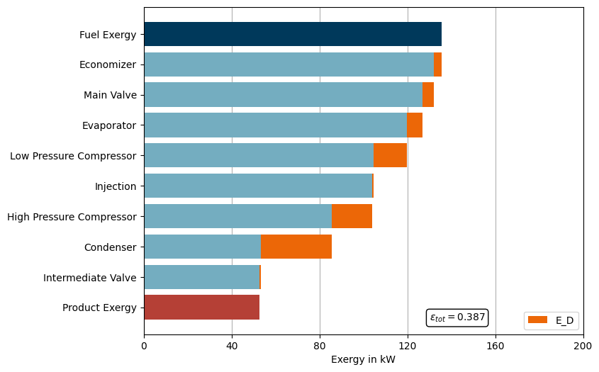
Explanation

• Verbesserung des COPs durch die doppelte Kompression.

• Exergie Wirkungsgrade der Komponenten

Economiser | E_F | E_P | E_D | epsilon Condenser | 8.451e+04 | 5.238e+04 | 3.213e+04 | 6.198e-01 HP Compressor | 9.351e+04 | 7.501e+04 | 1.850e+04 | 8.022e-01 LP Compressor | 6.420e+04 | 4.890e+04 | 1.530e+04 | 7.616e-01 Evaporator | 2.872e+04 | 2.177e+04 | 6.949e+03 | 7.581e-01 Main Valve | 3.372e+04 | 2.855e+04 | 5.164e+03 | 8.468e-01 Economizer | 4.942e+03 | 1.444e+03 | 3.498e+03 | 2.921e-01 Inter Valve | 7.912e+02 | nan | 7.912e+02 | nan
Injection | 1.371e+03 | 7.563e+02 | 6.150e+02 | 5.515e-01 Heat Consumer | 5.251e+04 | 5.239e+04 | 1.198e+02 | 9.977e-01 Sink Pump | 3.181e+02 | 2.490e+02 | 6.906e+01 | 7.829e-01 Source Pump | 4.455e+01 | 3.377e+01 | 1.078e+01 | 7.581e-01

Simple | E_F | E_P | E_D | epsilon Condenser | 7.188e+04 | 3.737e+04 | 3.451e+04 | 5.199e-01 Compressor | 1.649e+05 | 1.316e+05 | 3.324e+04 | 7.984e-01 Expansion Valve| 5.878e+04 | 4.154e+04 | 1.724e+04 | 7.067e-01 Evaporator | 4.086e+04 | 3.363e+04 | 7.223e+03 | 8.232e-01 Heat Consumer | 3.750e+04 | 3.738e+04 | 1.202e+02 | 9.968e-01 Sink Pump | 3.181e+02 | 2.471e+02 | 7.095e+01 | 7.769e-01 Source Pump | 4.420e+01 | 3.330e+01 | 1.089e+01 | 7.535e-01

Lessons Learned

• Lessons Learned 1

• Lessons Learned 2

• Lessons Learned 3