Compressed Air Production#

Fig. 11 Abstract model representation of a Compressor.#
Introduction#
In this example we are investigating the provision of compressed air. Compressed air is often required in technical systems, e.g. for process control, or as storage medium, i.e. in Compressed Air Energy Storage (CAES). To generate compressed air a compressor is required, which will (in the best case) compress the air in an isentropic process. The isentropic process is characterized by the fact, that the entropy does not change.
We can model such a process using CoolProp. For example, we want to compress 1.5 kg/s of air from the ambient state to a pressure of 10 bar. To calculate the energy consumed in the isentropic process, the energy balance introduced in eq. (16) can be simplified by removing the heat transfer term:
from CoolProp.CoolProp import PropsSI


T_amb = 20  # °C
p_amb = 1.01325  # bar
fluid = "air"
dot_m = 1.5

h_amb = PropsSI("H", "T", T_amb + 273.15, "P", p_amb * 1e5, fluid)
s_amb = PropsSI("S", "T", T_amb + 273.15, "P", p_amb * 1e5, fluid)

p_1 = p_amb
T_1 = T_amb

p_2 = 10

h_1 = h_amb
s_1 = s_amb
s_2 = s_1

h_2 = PropsSI("H", "S", s_1, "P", p_2 * 1e5, fluid)

dot_W = dot_m * (h_2 - h_1)

dot_W
407576.7496308336
We can define the exergy balance for the compressor at temperatures above the ambient temperature in the eqs. (25) and (26). With that definition it is possible to determine fuel, product and exergy destruction.
from utilities import calc_physical_exergy


exergy_fuel = dot_W

ex_1 = calc_physical_exergy(p_1 * 1e5, h_1, p_amb * 1e5, T_amb + 273.15, fluid)
ex_2 = calc_physical_exergy(p_2 * 1e5, h_2, p_amb * 1e5, T_amb + 273.15, fluid)

exergy_product = dot_m * (ex_2 - ex_1)

exergy_destruction = exergy_fuel - exergy_product

exergy_destruction
5.820766091346741e-10
First, we see that the exergy destruction is zero, which verifies our calculation: Since the isentropic process is adiabatic and reversible we have thermodynamically speaking an ideal process. Since such a component can only exist in theory, a reference figure is used to define how close an actual compressor is to the theoretical optimum: the isentropic efficiency \(\eta_\text{s,cmp}\) in eq. (27):
Exercises 1#
Assume you want to compress the same amount of air to the same pressure as in the example before:
What power does a compressor with an isentropic efficiency of 85 % consume?
How large is the exergy destruction?
How and why does the product exergy change?
What is the overall process exergy efficiency in both cases?
Solution 1#
To calculate the outlet state of the compressor with the isentropic efficiency of 85 % we have to first reorder the eq. (27) in a way, that the unknown outlet enthalpy can be calculated:
Then we create a function to calculate the enthalpy after isentropic compression \(h \left( p_2, s_1\right)\) and call it with the respective parameters.
def isentropic_outlet_enthalpy(p_1, h_1, p_2, fluid):
    s_1 = PropsSI("S", "P", p_1 , "H", h_1, fluid)
    h_2s = PropsSI("H", "P", p_2, "S", s_1, fluid)
    return h_2s


eta_s = 0.85

h_2_real = (isentropic_outlet_enthalpy(p_1 * 1e5, h_1, p_2 * 1e5, fluid) - h_1) / eta_s + h_1

dot_W_real = dot_m * (h_2_real - h_1)

dot_W_real / dot_W - 1
0.17647058823529416
We can see how the work required increases by about 17.65 %. Now let’s have a look at the exergy analysis. We can calculate the balance with the updated outlet state and have a look at the exergy destruction:
exergy_fuel_real = dot_W_real

ex_2_real = calc_physical_exergy(p_2 * 1e5, h_2_real, p_amb * 1e5, T_amb + 273.15, fluid)

exergy_product_real = dot_m * (ex_2_real - ex_1)

exergy_destruction_real = exergy_fuel_real - exergy_product_real

exergy_destruction_real
36204.98829636583
The exergy destruction is at 36205 W, the change of work transferred by the compressor (compared to the ideal compressor) is 71925 W. This may seem odd at the first glance. If the power input to the process has increased stronger than the exergy destruction, more product exergy must be available than before. We can verify this:
exergy_product_real - exergy_product
35720.320462017145
Looking at the exergy efficiency we can see, that the isentropic compressor provides 100 % efficiency. The real compressor induces exergy destruction, thus cannot have 100 % efficiency.
epsilon = exergy_product / dot_W
epsilon_real = exergy_product_real / dot_W_real
epsilon
0.9999999999999986
epsilon_real
0.9244946133954279
Overall process product#
We have learned how to run energy and exergy balances on a single compressor and found, that a less efficiency compressor consumes more power for the provision of the same mass flow at a specific pressure (obviously), but also that the product exergy increases the less efficient the compressor is.
This seems very counterintuitive as we always provide 1.5 kg/s compressed air at a pressure of 10 bar. However, we have not yet looked at the outlet temperature of the compressor. We can do that by calculating the temperature at the outlet pressure and the respective enthalpy.
T_2_is = PropsSI("T", "P", p_2 * 1e5, "H", h_2, fluid)
T_2_is - 273.15
286.660898246084
T_2 = PropsSI("T", "P", p_2 * 1e5, "H", h_2_real, fluid)
T_2 - 273.15
332.31621838839794
It becomes clear, that the outlet temperature rises with a lower isentropic efficiency of the compressor. Obviously, our total exergy changes, but we want to have a look at how the shares of physical and thermal exergy change.
Exercise 2#
Compare the mechanical and thermal exergy for the compressed air provided by the ideal and the real compressor.
Why does the mechanical exergy not change?
Solution 2#
We can make use of the exergy splitting to calculate thermal and mechanical exergy and specifically look at the mechanical exergy first: It does NOT change.
from utilities import calc_splitted_physical_exergy


ex_2_ideal_therm, ex_2_ideal_mech = calc_splitted_physical_exergy(p_2 * 1e5, h_2, p_amb * 1e5, T_amb + 273.15, fluid)
ex_2_therm, ex_2_mech = calc_splitted_physical_exergy(p_2 * 1e5, h_2_real, p_amb * 1e5, T_amb + 273.15, fluid)


ex_2_mech - ex_2_ideal_mech
0.0
That means the change in product exergy is purely due to a change in thermal exergy:
dot_m * (ex_2_therm - ex_2_ideal_therm)
35720.32046201713
exergy_product_real - exergy_product
35720.320462017145
What does this mean about the overall process product exergy? In our technical system we want to provide pneumatic energy. We cannot make use of the high temperature for this specific reason. Of course, one could use that thermal exergy to provide heat to other processes, but for now we want to focus on the provision of pressurized air. Thinking at this, the value of our process lies in the pressure of the air, not in the temperature. Therefore, we want to investigate more on this by defining a virtual process, which cools the pressurized air back to the ambient temperature without changing the pressure as illustrated in Fig. 12.

Fig. 12 Process representation of the compressor with virtual cooling of the compressed air.#
Exercise 3#
Balance the virtual process according to the flowsheet above assuming the temperature at point 3 is at the ambient temperature and the pressure does not change between the states 2 and 3.
Between the states 1 and 3
How does the enthalpy change?
How much energy is transferred overall?
How do mechanical and thermal exergy change?
Between the states 2 and 3
How much heat is transferred?
How much do mechanical and thermal exergy change?
How do the heat transfer and the change in thermal exergy connect?
Solution 3#
We have the following constraints in the compressed air system:
We have already calculated the enthalpy at the states 1 and 2. Therefore, we calculate the missing value of enthalpy at state 3 and find the change in enthalpy and the overall energy transfer between the states 1 and 3. Overall, the enthalpy changes by about -2.1 kJ/kg and the total energy transfer nets to -3.2 kW.
T_3 = T_1
p_3 = p_2
h_3 = PropsSI("H", "T", T_3 + 273.15, "P", p_3 * 1e5, "air")
h_3 - h_1
-2117.337343836669
dot_m * (h_3 - h_1)
-3176.0060157550033
For an outside observer not knowing about the specifics of the process, it seems as if the potential of the compressed air at the state 3 is lower than at the state 1. By calculating the exergy change we can however find, that the potential has actually increased.
Note
For completeness, we are also calculating the exergy of the state 1, which must be equal to zero, since we are in ambient state in that point.
ex_1_therm, ex_1_mech = calc_splitted_physical_exergy(p_1 * 1e5, h_1, p_amb * 1e5, T_amb +273.15, "air")
ex_3_therm, ex_3_mech = calc_splitted_physical_exergy(p_3 * 1e5, h_3, p_amb * 1e5, T_amb +273.15, "air")

(ex_3_therm + ex_3_mech) - (ex_1_therm + ex_1_mech)
192380.30251046058
We find the changes in the individual constituents of the exergy, the thermal exergy does obviously not change, because we are at ambient temperature in both cases. The mechanical exergy has however increased.
ex_3_therm - ex_1_therm
-9.331643013865686e-10
ex_3_mech - ex_1_mech
192380.3025104615
Next we have a look at the process between the states 2 and 3. First, we identify the amount of heat transferred. For that we have to make the energy balance of that process.
We can compare the amount of heat withdrawn with the change in exergy, which is the exergy destruction in the virtual cooling process. It becomes apparent, that the exergy destruction is lower than the heat transferred, because heat does not consist of pure exergy. And we can see, that the exergy destruction is purely caused by destruction of thermal exergy. The mechanical exergy does not change, because the pressure does not change.
dot_Q = dot_m * (h_3 - h_2)
dot_E_D = dot_m * (ex_3_therm + ex_3_mech - (ex_2_therm + ex_2_mech))
dot_Q
-410752.75564658863
dot_E_D
-154726.61632715934
ex_3_therm - ex_2_therm
-103151.07755143952
ex_3_mech - ex_2_mech
0.0
Improving the process#
To thermodynamically improve the process (minimizing the exergy destruction) we subdivide our compressor into two separate stages with intermittent cooling as shown in Fig. 13.

Fig. 13 Process representation of a compressor with two stages and intermittent cooling.#
Exercise 4#
Model the process of
compressing the ambient air to 3 bar,
cooling the air back to the ambient temperature and
compressing the air up to 10 bar.
Assume, that the isentropic efficiency of the two compressor stages is 85 %.
Then balance the process with energy and exergy:
How does the overall power requirement change compared to single stage compression?
How does the overall exergy destruction change compared to single stage compression?
Why is the overall exergy efficiency smaller in the two stage compressor, while less power is consumed than the single stage compression?
Solution 4#
To run the energy and exergy balances on the compressor with intermittent cooling, we first have to determine all missing values. We know the pressure in all points and the temperature at the inlet and at the outlet. With the isentropic efficiency definition from eq. (27) we can determine all enthalpies.
Next, we can calculate the total power input as well as define the overall process fuel exergy and product exergy in eqs. (30) and (31). Exergy losses, e.g. by leaking mass flow are not considered. The exergy destruction and exergy efficiency can then be calculated according to the theory (eqs. (32) and (33)).
eta_s = 0.85

p_amb = 1e5
T_amb = 25 + 273.15

p_1 = 1e5
p_2 = 3e5
p_3 = p_2
p_4 = 10e5

T_1 = 25 + 273.15
T_3 = T_1

h_1 = PropsSI("H", "T", T_1, "P", p_1, "air")
h_2 = (isentropic_outlet_enthalpy(p_1, h_1, p_2, fluid) - h_1) / eta_s + h_1
h_3 = PropsSI("H", "T", T_3, "P", p_3, "air")
h_4 = (isentropic_outlet_enthalpy(p_3, h_3, p_4, fluid) - h_3) / eta_s + h_3
The total electricity consumption of the compressor is achieved from the energy balance of the compressor. For the exergy analysis we follow the previous definitions.
dot_W_1 = dot_m * (h_2 - h_1)
dot_W_2 = dot_m * (h_4 - h_3)
ex_4 = calc_physical_exergy(p_4, h_4, p_amb, T_amb, "air")

E_F = dot_W_1 + dot_W_2
E_P = dot_m * ex_4
E_D = E_F - E_P
epsilon = E_P / E_F
We can have a look at the total power input and compare it to the single stage compressor power input. It is lower by about 14.07 %.
dot_W_1 + dot_W_2
412015.4274043005
dot_W_real
479502.058389216
Looking at the overall exergy destruction, we can see that it is higher for the intermittent cooling variant by about 40268 W. The reason for that is, that in our single stage compressor we considered the thermal exergy in the outlet stream as part of the product exergy.
E_D
76472.85486507835
Let us change this consideration: We add virtual cooling for both compressor variants at the end to make the product exergy comparable. First we implement it for the intermittent cooling variant.
T_5 = T_1
p_5 = p_4
h_5 = PropsSI("H", "T", T_5, "P", p_5, "air")
ex_5 = calc_physical_exergy(p_5, h_5, p_amb, T_amb, "air")

E_F = dot_W_1 + dot_W_2
E_P = dot_m * ex_5
E_D = E_F - E_P
epsilon = E_P / E_F
epsilon
0.7165625434300388
Then we can calculate the information for the single stage compression following the previous implementation.
p_2_single_stage = 10e5
p_3_single_stage = p_2_single_stage

h_2_single_stage = (isentropic_outlet_enthalpy(p_1, h_1, p_2_single_stage, fluid) - h_1) / eta_s + h_1
h_3_single_stage = PropsSI("H", "T", T_3, "P", p_3_single_stage, "air")

ex_3_single_stage = calc_physical_exergy(p_3_single_stage, h_3_single_stage, p_amb, T_amb, "air")

dot_W_single_stage = dot_m * (h_2_single_stage - h_1)

E_F_single_stage = dot_W_single_stage
E_P_single_stage = dot_m * ex_3_single_stage
E_D_single_stage = E_F_single_stage - E_P_single_stage
epsilon_single_stage = E_P_single_stage / E_F_single_stage
epsilon_single_stage
0.6008313425821769
We can see that the product exergy is equal.
E_P_single_stage == E_P
True
Assuming dissipative cooling for the intermittent cooling and the virtual cooling at the end of the process we can define the exergy balance for such components in eqs. (34) and (35). The product exergy is not defined, since there is no usable product in dissipative cooling.
Following this and the definitions for the single compressors, it is possible to calculate the component specific exergy destruction in the system and see how each component contributes to the overall exergy destruction of the system. This is a good starting point for process optimization, since we can determine which components have most optimization potential.
However, since we have to implement the balances for every component manually, with the use of a framework, i.e. TESPy, which already implemented this feature we can evaluate such systems much more time-efficiently.
Tip
A small introductory example on the concept and usage of TESPy is included in this section. You will find helpful links for more educational material on TESPy in that section. We recommend you get used to the API of TESPy before proceeding with the next exercise.
We can build a TESPy model for the single stage compression with virtual cooling at the end:
from tespy.components import Source, Sink, Compressor, HeatExchangerSimple
from tespy.connections import Connection, Bus
from tespy.networks import Network


nwk_single_stage = Network(fluids=["air"], p_unit="bar", T_unit="C")

compressor = Compressor("compressor")
cooler = HeatExchangerSimple("virtual cooling")
ambient_air = Source("ambient air")
compressed_air = Sink("compressed air")

c1 = Connection(ambient_air, "out1", compressor, "in1")
c2 = Connection(compressor, "out1", cooler, "in1")
c3 = Connection(cooler, "out1", compressed_air, "in1")

nwk_single_stage.add_conns(c1, c2, c3)
After setting up the system’s topology we can specify the process and component parameters.
c1.set_attr(fluid={"air": 1}, p=1, T=25, m=dot_m)
c3.set_attr(p=10, T=25)

cooler.set_attr(pr=1)
compressor.set_attr(eta_s=eta_s)
Then we solve the model. Results can be obtained from the .results attribute of the network or directly from the
connection and component objects.
nwk_single_stage.solve("design")
 iter  | residual   | progress   | massflow   | pressure   | enthalpy   | fluid      |
-------+------------+------------+------------+------------+------------+------------+
 1     | 9.06e+05   | 50 %       | 2.79e-01   | 9.00e+05   | 1.03e+06   | 0.00e+00   |
 2     | 4.92e+05   | 50 %       | 0.00e+00   | 0.00e+00   | 5.78e+05   | 0.00e+00   |
 3     | 1.10e-12   | 53 %       | 0.00e+00   | 0.00e+00   | 1.15e-09   | 0.00e+00   |
 4     | 9.31e-10   | 53 %       | 0.00e+00   | 0.00e+00   | 1.74e-09   | 0.00e+00   |
 5     | 2.33e-10   | 53 %       | 0.00e+00   | 0.00e+00   | 1.23e-09   | 0.00e+00   |
Total iterations: 5, Calculation time: 0.01 s, Iterations per second: 549.24
With that, we can verify our own implementation, e.g. total enthalpy change, power input or heat extraction.
round(dot_W_single_stage) == round(compressor.P.val)
True
round(h_3_single_stage - h_1) == round(c3.h.val_SI - c1.h.val_SI)
True
round(dot_m * (h_3_single_stage - h_2_single_stage)) == round(cooler.Q.val)
True
We can set up the exergy analysis easily. Overall fuel and product exergy are defined with Bus objects.
from tespy.tools import ExergyAnalysis


fuel_exergy = Bus("fuel exergy")
fuel_exergy.add_comps({"comp": compressor, "base": "bus"})

product_exergy = Bus("product exergy")
product_exergy.add_comps({"comp": compressed_air})

nwk_single_stage.add_busses(fuel_exergy, product_exergy)
ean_single_stage = ExergyAnalysis(nwk_single_stage, E_F=[fuel_exergy], E_P=[product_exergy])
ean_single_stage.analyse(pamb=1, Tamb=25)
The .network_data attribute stores the result of the overall system. The .connection_data the connections’ exergy
flows and the .component_data the components’ results. For example, we can check the overall exergy efficiency.
round(ean_single_stage.network_data.loc["epsilon"], 6) == round(epsilon_single_stage, 6)
True
Exercise 5#
Build a TESPy model for the intermittent cooling compressor process with the virtual cooling at the end.
Verify the results of your own implementation with the TESPy implementation.
Set up and run the exergy analysis.
Vary the intermediate pressure and calculate the process exergy efficiency for a pressure range of 2 bar to 9 bar. Make a plot that shows the exergy efficiency for every intermediate pressure value.
Solution 5#
We build the model similarly as the single stage model. First we set up the components and the connections:
from tespy.components import Source, Sink, Compressor, HeatExchangerSimple
from tespy.connections import Connection, Bus
from tespy.networks import Network


nwk_two_stage = Network(fluids=["air"], p_unit="bar", T_unit="C")

compressor_stage_1 = Compressor("compressor stage 1")
compressor_stage_2 = Compressor("compressor stage 2")
intermittent_cooler = HeatExchangerSimple("intermittent cooling")
cooler = HeatExchangerSimple("virtual cooling")
ambient_air = Source("ambient air")
compressed_air = Sink("compressed air")

c1 = Connection(ambient_air, "out1", compressor_stage_1, "in1", label="1")
c2 = Connection(compressor_stage_1, "out1", intermittent_cooler, "in1", label="2")
c3 = Connection(intermittent_cooler, "out1", compressor_stage_2, "in1", label="3")
c4 = Connection(compressor_stage_2, "out1", cooler, "in1", label="4")
c5 = Connection(cooler, "out1", compressed_air, "in1", label="5")

nwk_two_stage.add_conns(c1, c2, c3, c4, c5)
The next step is to specify the process and component information.
c1.set_attr(fluid={"air": 1}, p=1, T=25, m=dot_m)
c3.set_attr(p=3, T=25)
c5.set_attr(p=10, T=25)

intermittent_cooler.set_attr(pr=1)
cooler.set_attr(pr=1)

compressor_stage_1.set_attr(eta_s=eta_s)
compressor_stage_2.set_attr(eta_s=eta_s)
We can solve the model and then verify if the total compression power consumption is identical in our TESPy model and the previous manual implementation.
nwk_two_stage.solve("design")
 iter  | residual   | progress   | massflow   | pressure   | enthalpy   | fluid      |
-------+------------+------------+------------+------------+------------+------------+
 1     | 9.28e+05   | 50 %       | 4.70e-01   | 9.22e+05   | 7.63e+05   | 0.00e+00   |
 2     | 3.63e+05   | 50 %       | 0.00e+00   | 0.00e+00   | 4.27e+05   | 0.00e+00   |
 3     | 6.32e-10   | 53 %       | 0.00e+00   | 0.00e+00   | 1.45e-09   | 0.00e+00   |
 4     | 3.52e-10   | 53 %       | 0.00e+00   | 0.00e+00   | 1.30e-09   | 0.00e+00   |
 5     | 3.39e-10   | 53 %       | 0.00e+00   | 0.00e+00   | 1.19e-09   | 0.00e+00   |
Total iterations: 5, Calculation time: 0.02 s, Iterations per second: 331.89
round(dot_W_1 + dot_W_2) == round(compressor_stage_1.P.val + compressor_stage_2.P.val)
True
The exergy analysis setup is straight forward again:
Define the busses for fuel and product exergy
Add them to the network
Run the analysis
Then we can again verify if our TESPy model computes the same output as the manual implementation.
fuel_exergy = Bus("fuel exergy")
fuel_exergy.add_comps(
    {"comp": compressor_stage_1, "base": "bus"},
    {"comp": compressor_stage_2, "base": "bus"},
)

product_exergy = Bus("product exergy")
product_exergy.add_comps({"comp": compressed_air})

nwk_two_stage.add_busses(fuel_exergy, product_exergy)
ean_two_stage = ExergyAnalysis(nwk_two_stage, E_F=[fuel_exergy], E_P=[product_exergy])
ean_two_stage.analyse(pamb=1, Tamb=25)
round(ean_two_stage.network_data.loc["epsilon"], 6) == round(epsilon, 6)
True
To investigate the effect of the intermediate pressure value on the exergy efficiency of the overall process we create a loop over the defined pressure range in which
we set the intermediate pressure on the respective connection,
solve the model,
reanalyze the network and
store the exergy efficiency result.
Then we can plot the result in Fig. 14. We can see, that there is a clear optimum at around 3.14 bar.
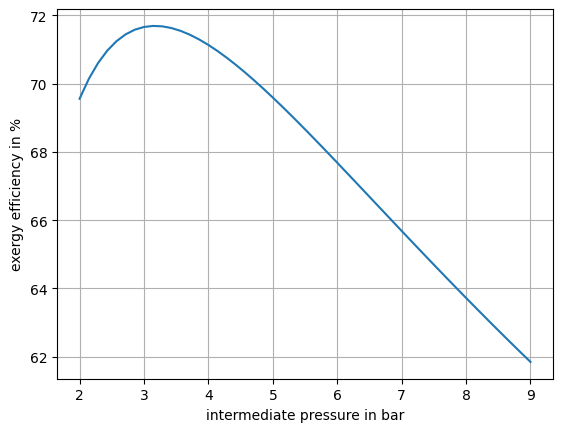
Fig. 14 Exergy efficiency of the overall process as function of the intermediate pressure.#
import numpy as np


p_range = np.linspace(2, 9)
epsilon_range = []
nwk_two_stage.set_attr(iterinfo=False)

for p in p_range:
    c3.set_attr(p=p)
    nwk_two_stage.solve("design")
    ean_two_stage.analyse(pamb=1, Tamb=25)

    epsilon_range += [ean_two_stage.network_data.loc["epsilon"] * 100]
from matplotlib import pyplot as plt


fig, ax = plt.subplots(1)

ax.plot(p_range, epsilon_range)

ax.set_ylabel("exergy efficiency in %")
ax.set_xlabel("intermediate pressure in bar")

ax.grid()
ax.set_axisbelow(True)

plt.close()
Lessons Learned#
…
…