Adiabatic Pipe Flow

In this section we will have a look at an adiabatic pipe with pressure losses occurring. With the first law of thermodynamics we cannot see a change in energy, exergy analysis can reveal the thermodynamic losses.

Introduction

Consider a well insulated pipeline transporting steam as shown in the figure below.

Fig. 3 Abstract model of the well insulated steam pipeline.

Measurement data are obtained at the inlet and the outlet of the pipeline:

Parameter	Location	Value	Unit
Temperature	Inlet	195	°C
	Outlet	184.4	°C
Pressure	Inlet	10	bar
	Outlet	6	bar
Mass flow	Inlet	1.2	kg/s

First, we can set up the energy balance equation of the thermodynamic open system, where the work \(\dot W\) and heat \(\dot Q\) transferred change the enthalpy \(h\) of a mass flow \(\dot m\) from a state 1 to a different state 2:

(16)\[ \dot W + \dot Q = \dot m \cdot \left(h_2 - h_1\right)\]

Since a pipe does not transfer work to the fluid, work transferred can be considered equal to zero. Thus, the specific heat transferred can be calculated by the change of enthalpy. Since the pipeline is well insulated, the value should be rather small.

(17)\[\begin{split} \frac{\dot Q}{\dot m} = h_2 - h_1\\\end{split}\]

To do that computationally, we first import the PropsSI function from CoolProp and then insert the values from the table above.

from CoolProp.CoolProp import PropsSI as PSI


fluid = "water"

p_in = 10 * 1e5
T_in = 195 + 273.15
h_in = PSI("H", "P", p_in, "T", T_in, fluid)

p_out = 6 * 1e5
T_out = 184.4 + 273.15
h_out = PSI("H", "P", p_out, "T", T_out, fluid)

q = h_out - h_in
q

-32.01454686373472

Attention

As we expected the specific heat transferred is very low. Therefore we will make an assumption, that the pipeline can be considered adiabatic for further calculations. If transferred work and heat are both zero, the change in enthalpy will therefore be zero as well:

\[ h_2 = h_1\]

We can also double-check this, by calculating the outlet temperature at the measured outlet pressure and with the assumption of non-changing enthalpy. Note that it is only slightly different:

h_out = h_in
PSI("T", "P", p_out, "H", h_out, fluid) - 273.15

184.4142164685412

We have seen, that no energy has been transferred from the pipe to the ambient. Does that mean, we can revert the process? Obviously, that does not seem natural, as you cannot change the pressure of the fluid at the outlet back to the inlet pressure without adding any energy. That means, while we have not lost any energy to the ambient, the energy must have become less valuable.

Exergy Analysis

In this chapter, we will learn, how the described change in quality of energy can be made visible using Second Law analysis. To do that, we calculate the exergy of the fluid at the inlet and at the outlet of the pipe. First, we define a function, that follows the definition of physical exergy in eq. (4) without splitting physical exergy into mechanical and thermal share. Chemical exergy can be ignored in this application, since no chemical reaction processes take place.

The function calc_physical_exergy will take pressure and enthalpy of a fluid and calculate the thermal and the mechanical part of the physical exergy.

def calc_physical_exergy(p, h, p0, T0, fluid):
    r"""Calculate specific physical exergy."""
    s = PSI("S", "P", p, "H", h, fluid)    
    h0 = PSI("H", "P", p0, "T", T0, fluid)
    s0 = PSI("S", "P", p0, "T", T0, fluid)
    
    ex = (h - h0) - T0 * (s - s0)
    return ex

Then, we can define an (arbitrary) ambient state and calculate the exergy and the inlet and the outlet state.

p0 = 1.01325 * 1e5
T0 = 20 + 273.15
m = 1

ex_in = calc_physical_exergy(p_in, h_in, p0, T0, fluid) * m
ex_in

863747.8363819825

ex_out = calc_physical_exergy(p_out, h_out, p0, T0, fluid) * m
ex_out

797952.1230949757

With that, we can set up the exergy balance equation (eq. (18)). The adiabatic pipe component does not serve any other purpose than transporting a fluid from one place to another. Energetically, the adiabatic pipe is a “useless” component, which means, that the exergy product is not defined. The fuel exergy is then the inlet exergy, the exergy destruction the difference between inlet and outlet exergy:

(18)\[\begin{split} \dot E_F=\dot m \cdot e^\text{PH}_\text{in}\\ \dot E_D=\dot m \cdot \left(e^\text{PH}_\text{in} - e^\text{PH}_\text{out}\right)\end{split}\]

exergy_destruction = ex_in - ex_out
exergy_destruction

65795.71328700683

exergy_destruction_rate = exergy_destruction / ex_in
exergy_destruction_rate

0.07617467797384957

We see that a total of 65796 J/kg is destroyed, which corresponds to an exergy destruction rate of about 7.62 %.

Exercises part 1

With the information from the sections above:

1. Calculate the total exergy destruction and the exergy efficiency of the pipe flow for varying outlet pressures in a range from the ambient pressure to the inlet pressure.

   • As a function of the pipe pressure drop (x-axis) plot the:

     • exergy destruction (y-axis).

     • exergy destruction ratio (y-axis).

2. What could be the reason, the exergy destruction ratio not equal to 100 %, when the pressure at the pipeline outlet is equal to the ambient pressure? What are the relevant equations in the theory (section exergy analysis)?

Solution 1

We can use numpy to create a vector of outlet pressure values and then calculate the outlet exergy vector. The inlet exergy does not change for all values. Then with matplotlib we can create two subplots sharing the same x-axis (i.e. the pressure range) and plot the exergy destruction and the exergy efficiency.

Show code cell content Hide code cell content

import numpy as np
from matplotlib import pyplot as plt

outlet_pressure_range = np.linspace(10, p0 / 1e5) * 1e5
pressure_difference_range = p_in - outlet_pressure_range
ex_out = calc_physical_exergy(outlet_pressure_range, h_out, p0, T0, fluid) * m
ex_in = calc_physical_exergy(p_in, h_in, p0, T0, fluid) * m


fig, ax = plt.subplots(2, sharex=True)

ax[0].plot(pressure_difference_range / 1e5, (ex_in - ex_out) / 1e3)
ax[1].plot(pressure_difference_range / 1e5, (ex_in - ex_out) / ex_in * 100)

ax[0].set_ylabel("Exergy destruction in kW")
ax[1].set_ylabel("Exergy destruction ratio in %")
ax[1].set_xlabel("Pipe pressure loss in bar")

_ = [(a.grid(), a.set_axisbelow(True)) for a in ax]

plt.close()

Result

From Fig. 4 we can see, that the destruction of exergy obviously depends on the change of pressure in the pipe. The higher the pressure loss, the higher the destruction of exergy. The change in exergy destruction does increase the higher the pressure loss is.

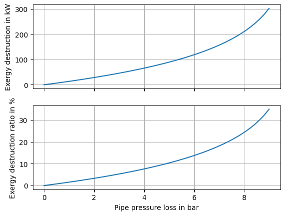
Fig. 4 Exergy destruction and exergy destruction ratio as function of the pipe’s outlet pressure.

Solution 2

From Fig. 4 we can also see, that at a pressure loss of about 9 bars, i.e. when the outlet pressure is at the ambient state, the exergy destruction rate is not at 100 %. This means there must still be exergy in the outlet flow. We can check that, by looking at the last value in the ex_out vector.

Show code cell content Hide code cell content

ex_out_p_ambient = ex_out[-1]
ex_out_p_ambient

561738.2486228282

Exergy is a function of pressure and temperature (difference to ambient state), we can have a look at the outlet temperature, when the steam is throttled to the ambient pressure without changing enthalpy:

Show code cell content Hide code cell content

T_out_at_p_ambient = PSI("T", "P", p0, "H", h_out, fluid) - 273.15
T_out_at_p_ambient

169.94765628665198

The temperature is higher than the ambient state, thus we can expect that there is still some exergy remaining in the temperature of the fluid. With the learnings from the introduction chapter, i.e. that physical exergy consists of the two components

• mechanical exergy and

• thermal exergy,

we find, that either the thermal or the mechanical exergy (or both) is not zero at the outlet.

Exercises part 2

3. Create a function that splits the physical exergy in its thermal and mechanical shares according to eq. (5) and eq. (6).

   • Verify that your function produces the same result as the function defined earlier.

   • Create a plot that shows, how thermal and mechanical exergy are affected by the pressure change within the specified pressure range.

   • What is the thermal, and what is the mechanical exergy of the steam, when the pressure at the outlet is at ambient state?

4. Instead of a steam flow consider flow of hot air:

   • Create a plot with exergy destruction and exergy destruction ratio of both air and water inside the same subplots.

   • Why is the influence of the pressure on the exergy destruction ratio of the air flow much higher than on the exergy efficiency of the steam flow?

Solution 3

First we define a new function that returns the thermal and the mechanical share of exergy according the equations (5), (6) and (7). Then we can calculate the share of thermal and mechanical exergy at the inlet state of the air pipe and validate, if the sum of both shares is equal to the result from our first implementation of the physical exergy:

Show code cell content Hide code cell content

def calc_splitted_physical_exergy(p, h, p0, T0, fluid):
    r"""Calculate specific physical exergy according to splitting rule."""
    s = PSI("S", "P", p, "H", h, fluid)
    
    h_T0_p = PSI("H", "P", p, "T", T0, fluid)
    s_T0_p = PSI("S", "P", p, "T", T0, fluid)
    
    ex_therm = (h - h_T0_p) - T0 * (s - s_T0_p)
    
    h0 = PSI("H", "P", p0, "T", T0, fluid)
    s0 = PSI("S", "P", p0, "T", T0, fluid)
    
    ex_mech = (h_T0_p - h0) - T0 * (s_T0_p - s0)
    return ex_therm, ex_mech

ex_T_in, ex_M_in = calc_splitted_physical_exergy(p_in, h_in, p0, T0, "water")

round(ex_T_in + ex_M_in, 3) == round(calc_physical_exergy(p_in, h_in, p0, T0, "water"), 3)  # should return True

True

In the next step we calculate the thermal and mechanical exergy for all pressure range for the outlet state as we did before. Then, we can make two subplots, which show the change in thermal exergy and the change in mechanical exergy.

Show code cell content Hide code cell content

ex_T_out, ex_M_out = calc_splitted_physical_exergy(outlet_pressure_range, h_out, p0, T0, "water") * m


fig, ax = plt.subplots(2, sharex=True)

ax[0].plot(pressure_difference_range / 1e5, (ex_T_in - ex_T_out) / 1e3)
ax[1].plot(pressure_difference_range / 1e5, (ex_M_in - ex_M_out) / 1e3)

ax[0].set_ylabel("$\Delta \\mathrm{Ex}^\\mathrm{T}$ in kW")
ax[1].set_ylabel("$\Delta \\mathrm{Ex}^\\mathrm{M}$ in kW")
ax[1].set_xlabel("Pipe pressure loss in bar")

_ = [(a.grid(), a.set_axisbelow(True)) for a in ax]

plt.close()

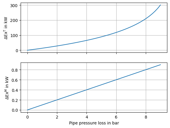
Fig. 5 Change in thermal and mechanical exergy of the steam pipe flow depending on the pressure change.

In Fig. 5 we can see the change of thermal and of mechanical exergy in the pipe flow at the different pressure losses. Note, the different scales:

• The thermal exergy changes by up to 300 kW.

• The mechanical exergy changes only by about 0.9 kW at maximum.

Obviously, the much more thermal exergy is destroyed in the process than mechanical exergy, although only the pressure changes. This is because expansion of the steam causes a drop in temperature as well (as we have seen in the solution 2). The reason, why we see such a small change in mechanical exergy can be seen, when we have a look at the shares of thermal and mechanical exergies in the inlet state and the outlet state at ambient pressure. We can create a bar diagram for both states in Fig. 6. The exergy is nearly pure thermal exergy.

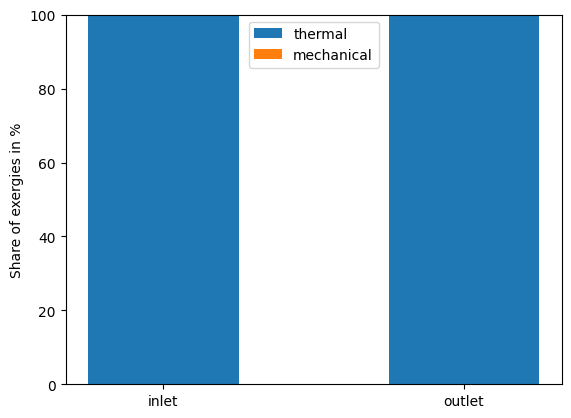
Fig. 6 Shares of thermal and mechanical exergy at the inlet and the outlet state at ambient pressure.

Show code cell content Hide code cell content

fig, ax = plt.subplots(1)

thermal = np.array([ex_T_in / ex_in, ex_T_out[-1] / ex_out[-1]]) * 100
mechanical = np.array([ex_M_in / ex_in, ex_M_out[-1] / ex_out[-1]]) * 100

ax.bar(["inlet", "outlet"], thermal, 0.5, label="thermal")
ax.bar(["inlet", "outlet"], mechanical, 0.5, label="mechanical", bottom=thermal)
ax.legend(loc=9)

ax.set_ylabel("Share of exergies in %")

plt.close()

Finally, we can verify the value of mechanical exergy of the steam at ambient pressure:

Show code cell content Hide code cell content

ex_M_out[-1]

0.0

Solution 4

We can build the same setup for the air flow using the defined inlet state. Since the enthalpy at the inlet is not the same as the enthalpy of water, we need to recalculate that value.

In the plots we plot the air and steam exergy destruction and efficiency into the same subplots and label them for the legend.

Show code cell content Hide code cell content

fluid = "air"
h_in_air = PSI("H", "T", T_in, "P", p_in, fluid)
h_out_air = h_in_air

ex_out_air = calc_physical_exergy(outlet_pressure_range, h_out_air, p0, T0, fluid)
ex_in_air = calc_physical_exergy(p_in, h_in_air, p0, T0, fluid)


fig, ax = plt.subplots(2, sharex=True)

ax[0].plot(pressure_difference_range / 1e5, (ex_in - ex_out) / 1e3, label="water")
ax[0].plot(pressure_difference_range / 1e5, (ex_in_air - ex_out_air) / 1e3, label="air")

ax[1].plot(pressure_difference_range / 1e5, (ex_in - ex_out) / ex_in * 100)
ax[1].plot(pressure_difference_range / 1e5, (ex_in_air - ex_out_air) / ex_in_air * 100)

ax[0].set_ylabel("Exergy destruction in kW")
ax[1].set_ylabel("Exergy destruction rate in %")
ax[1].set_xlabel("Pressure drop in bar")

ax[0].legend()
_ = [(a.grid(), a.set_axisbelow(True)) for a in ax]

plt.close()

In the first subplot of Fig. 7 we can see that in the steam flow the exergy destruction is higher by a factor of about 1.5. This ratio can be verified by checking Fig. 8. This displays the ratio over the pressure range, and we can see the ratio is merely affected by pressure.

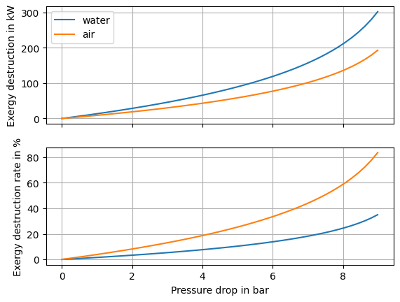
Fig. 7 Exergy destruction and exergy destruction share for the adiabatic steam and air flows.

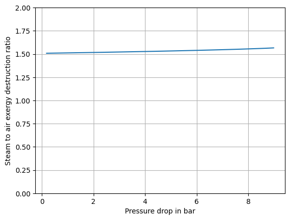
Fig. 8 Ratio of exergy destruction of steam to exergy destruction of air.

While the exergy destruction is higher for the steam flow, we see in the second subplot of Fig. 7 that the exergy destruction as share of the inlet exergy is much higher for air. When the pressure drops to ambient state pressure, more than 80 % of exergy of the air are destroyed. To understand why this is the case, we can again have a look at the shares of mechanical and thermal exergy for the air stream. We do this for the “extreme” case with the outlet pressure at ambient state, i.e. when all mechanical exergy is lost. The Fig. 6 displays the result.

Show code cell content Hide code cell content

fig, ax = plt.subplots(1)

ax.plot(pressure_difference_range / 1e5, (ex_in - ex_out) / (ex_in_air - ex_out_air))

ax.set_ylim([0, 2])
ax.set_ylabel("Steam to air exergy destruction ratio")
ax.set_xlabel("Pressure drop in bar")

_ = ax.grid(), ax.set_axisbelow(True)

plt.close()

/tmp/ipykernel_1951/3922793100.py:3: RuntimeWarning: invalid value encountered in divide
  ax.plot(pressure_difference_range / 1e5, (ex_in - ex_out) / (ex_in_air - ex_out_air))

Show code cell content Hide code cell content

ex_T_in_air, ex_M_in_air = calc_splitted_physical_exergy(p_in, h_in_air, p0, T0, fluid)
ex_T_out_air, ex_M_out_air = calc_splitted_physical_exergy(outlet_pressure_range, h_out_air, p0, T0, fluid)

fig, ax = plt.subplots(1)

thermal = np.array([ex_T_in_air / ex_in_air, ex_T_out_air[-1] / ex_out_air[-1]]) * 100
mechanical = np.array([ex_M_in_air / ex_in_air, ex_M_out_air[-1] / ex_out_air[-1]]) * 100

ax.bar(["inlet", "outlet"], thermal, 0.5, label="thermal")
ax.bar(["inlet", "outlet"], mechanical, 0.5, label="mechanical", bottom=thermal)
ax.legend(loc=9)

ax.set_ylabel("Share of exergies in %")

plt.close()

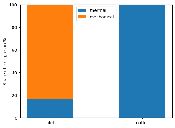
Fig. 9 Change in thermal and mechanical exergy of the air pipe flow depending on the pressure change.

In the figure above we can see that

• all mechanical exergy is destroyed when expanding to ambient pressure (as expected)

• the share of mechanical exergy at the air pipe inlet is about 87 %, thus a higher share of exergy of the inlet exergy is destroyed in the air stream.

Finally, we can check, how thermal exergy changes in case of the air flow and see, that only 0.5 kW of thermal exergy is lost.

Show code cell content Hide code cell content

ex_T_in_air - ex_T_out_air[-1]

499.4708984364988

Lessons Learned

• Physical exergy of a mass flow can be split into a thermal and a mechanical share.

• At the same pressure and temperature, the shares of the exergy depend on the working fluid.