Gas Turbine#
In this section we will be investigating gas turbine cycles using TESPy. In the first step the ideal Brayton cycle is modeled. The ideal Brayton cycle consists of three subprocesses, i.e. isentropic compression, isobaric heat transfer and isentropic expansion (see Fig. 15). Next, we are comparing the cycle to the open cycle gas turbine, which instead of isobaric heat transfer uses a combustion chamber.
Ideal Brayton Cycle#
The flowsheet of the Brayton cycle is shown in Fig. 15. Based on the flowsheet we can calculate the thermal efficiency of the cycle using eq. (36). For the exergy analysis we have to define the plant’s fuel and product exergy as well as the exergy losses in eqs. (37), (38) and (39).

Fig. 15 Flow sheet of the Brayton cycle.#
Table 1 indicates the parameter settings for the Brayton cycle for the initial setup.
Location |
Parameter |
Value |
Unit |
|---|---|---|---|
Compressor |
Isentropic efficiency |
100 |
% |
Pressure ratio |
10 |
||
Heater |
Pressure ratio |
1 |
|
Turbine |
Isentropic efficiency |
100 |
% |
Generator |
Total power output |
-100 |
MW |
1 |
Pressure |
1.013 |
bar |
Temperature |
25 |
°C |
|
3 |
Temperature |
1400 |
°C |
4 |
Pressure |
1.013 |
bar |
Exercise 1#
Build the TESPy model according to the flowsheet of the ideal Brayton cycle and its specifications shown in Table 1:
Calculate the thermal efficiency of the process.
Add the setup for the exergy analysis and run it:
What is the total exergy efficiency?
What is the total exergy destruction?
What are the exergy losses to the ambient?
Why is it impossible to reach an exergy efficiency of 100 % even with ideal components?
Solution 1#
We can set up the plant with standard components. The heater of the Brayton cycle can be represented by the
HeatExchangerSimple component.
from tespy.components import Source, Sink, Compressor, Turbine, HeatExchangerSimple
from tespy.connections import Connection, Bus
from tespy.networks import Network
from tespy.tools import ExergyAnalysis


nwk = Network(fluids=["Air"], p_unit="bar", T_unit="C", iterinfo=False)

p0 = 1.013
T0 = 25

so = Source("air intake")
cp = Compressor("compressor")
hi = HeatExchangerSimple("heater")
tu = Turbine("turbine")
si = Sink("air outlet")

c1 = Connection(so, "out1", cp, "in1", label="1")
c2 = Connection(cp, "out1", hi, "in1", label="2")
c3 = Connection(hi, "out1", tu, "in1", label="3")
c4 = Connection(tu, "out1", si, "in1", label="4")

nwk.add_conns(c1, c2, c3, c4)

power_output = Bus("power output")
power_output.add_comps(
    {"comp": cp, "base": "bus"},
    {"comp": tu, "base": "component"}
)

heat_input = Bus("heat input")
heat_input.add_comps(
    {"comp": hi, "base": "bus"},
)

chimney = Bus("chimney")
chimney.add_comps(
    {"comp": si, "base": "component"}
)
nwk.add_busses(power_output, heat_input, chimney)

c1.set_attr(fluid={"Air": 1}, p=p0, T=T0)
c3.set_attr(T=1400)
c4.set_attr(p=p0)

cp.set_attr(eta_s=1, pr=10)
hi.set_attr(pr=1)
tu.set_attr(eta_s=1)

power_output.set_attr(P=-100e6)

nwk.solve("design")

thermal_efficiency = abs(power_output.P.val) / heat_input.P.val

ean = ExergyAnalysis(nwk, E_F=[heat_input], E_P=[power_output], E_L=[chimney])

ean.analyse(p0, T0)

brayton_connections = nwk.results["Connection"].copy()
The cycle’s efficiency is at about 45.04 %, with an exergy efficiency of
63.14 %. We can extract the plant’s overall exergy analysis results from the
network_data attribute:
ean.network_data.to_frame().transpose().rename({0: "value"})
| E_F | E_P | E_D | E_L | epsilon | |
|---|---|---|---|---|---|
| value | 1.583699e+08 | 100000000.0 | 4.470348e-08 | 5.836990e+07 | 0.631433 |
As expected no exergy is destroyed in our setup, because the compressor and the turbine are isentropic components and the heat input is isobaric. However, our exergy efficiency is still not 100 %. The reason for this is, that the flue gas leaving the cycle to the ambient still contains exergy. The stream of physical exergy is therefore lost:
c4.Ex_physical
58369903.436568305
Open Cycle Gas Turbine#
In the second part of this section we are switching our investigation to an actual open cycle gas turbine system with combustion of fuel as indicated in Fig. 16. All relevant component and process parameters are indicated in Table 2. As fuel, we are going to use pure methane.

Fig. 16 Flow sheet of the open cycle gas turbine.#
Location |
Parameter |
Value |
Unit |
|---|---|---|---|
Compressor |
Isentropic efficiency |
100 |
% |
Pressure ratio |
10 |
||
Heater |
Pressure ratio |
1 |
|
Turbine |
Isentropic efficiency |
100 |
% |
Generator |
Total power output |
-100 |
MW |
Combustion Chamber |
Efficiency (thermal insulation) |
100 |
% |
Pressure losses |
0 |
% |
|
1 |
Pressure |
1.013 |
bar |
Temperature |
25 |
°C |
|
3 |
Temperature |
1400 |
°C |
4 |
Pressure |
1.013 |
bar |
5 |
Pressure |
\(p_\text{3} + 1\) |
bar |
In contrast to the previous exercise we have to model the air composition component wise in this example. We are going
to use an additional source for the fuel and the DiabaticCombustionChamber to make accounting of heat and pressure
losses in the combustion process possible. The topology can be built according to the flowsheet. A power output bus is
added to the network, which sums the power generation of the turbine with the power consumption of the compressor. The
net power can then be specified to that bus.
from tespy.components import Source, Sink, Compressor, Turbine, DiabaticCombustionChamber
from tespy.connections import Connection, Bus, Ref
from tespy.networks import Network
from tespy.tools import ExergyAnalysis


nwk = Network(fluids=["O2", "H2O", "CO2", "N2", "Ar", "CH4"], p_unit="bar", T_unit="C", iterinfo=False)

fuel = Source("methane source")
so = Source("air intake")
cp = Compressor("compressor")
dcc = DiabaticCombustionChamber("combustion chamber")
tu = Turbine("turbine")
si = Sink("air outlet")

c1 = Connection(so, "out1", cp, "in1", label="1")
c2 = Connection(cp, "out1", dcc, "in1", label="2")
c3 = Connection(dcc, "out1", tu, "in1", label="3")
c4 = Connection(tu, "out1", si, "in1", label="4")

c5 = Connection(fuel, "out1", dcc, "in2", label="5")

nwk.add_conns(c1, c2, c3, c4, c5)

power_output = Bus("power output")
power_output.add_comps(
    {"comp": cp, "base": "bus"},
    {"comp": tu, "base": "component"}
)
nwk.add_busses(power_output)
Then we make the parameter specifications. We have to provide component wise composition of the air, since the combustion process relies on the oxygen mass fraction in the ambient air. The same is then true for the fuel, here all mass fractions are zero except for the methane mass fraction. We can specify the total power output on the bus.
c1.set_attr(fluid={"N2": 0.7551, "O2": 0.2314, "Ar": 0.0129, "H2O": 0, "CO2": 0.0006, "CH4": 0}, p=p0, T=T0)
c3.set_attr(T=1400)
c4.set_attr(p=p0)

c5.set_attr(fluid={"N2": 0, "O2": 0, "Ar": 0, "H2O": 0, "CO2": 0, "CH4": 1}, p=Ref(c3, 1, 1), T=T0)

cp.set_attr(eta_s=1, pr=10)
dcc.set_attr(pr=1, eta=1)
tu.set_attr(eta_s=1)

power_output.set_attr(P=-100e6)
We can run the simulation and calculate the thermal efficiency. It is at 43.91 %, thus a little lower than in the ideal Brayton process.
nwk.solve("design")

thermal_efficiency_gt = abs(power_output.P.val) / (c5.m.val_SI * dcc.fuels["CH4"]["LHV"])
glue("gt-thermal-efficiency", round(thermal_efficiency_gt * 100, 2), display=False)
Exercise 2#
Make a comparison of the results between the Brayton and gas turbine cycle:
Air mass flow
Compressor outlet temperature
Turbine outlet temperature
Total heat input and thermal efficiency
How can the deviations be explained?
Solution 2#
For the comparison of the results between the two cycles, we have saved all connection information from the Brayton cycle in a dataframe. We can then subtract the results dataframes from each other. Rows and columns with missing values are dropped and only absolute properties (mass flow, temperature and pressure) are kept in the dataframe.
The relative deviation can then be calculated by dividing the absolute deviation by the results of the gas turbine cycle simulation.
deviation_abs = (brayton_connections - nwk.results["Connection"]).dropna(axis=1, how="all").dropna(how="all")[["T", "m", "p"]]
(deviation_abs / nwk.results["Connection"]).dropna(axis=1, how="all").dropna(how="all")
| T | m | p | |
|---|---|---|---|
| 1 | -2.273737e-15 | 0.099597 | 2.191951e-16 |
| 2 | 6.095697e-04 | 0.099597 | 0.000000e+00 |
| 3 | 1.143365e-13 | 0.068955 | 0.000000e+00 |
| 4 | -4.343118e-02 | 0.068955 | 0.000000e+00 |
We can see, that the temperature values deviate by a very small margin. The compressor inlet temperature is 0.06 % higher in the Brayton cycle than in the gas turbine cycle, the turbine outlet temperature is lower by about 4 %. Much higher deviation can be observed in the mass flow: Here the Brayton cycle requires 10 % more air mass flow and nearly 7 % more flue gas mass flow. The pressure values do not deviate.
Exercise 4#
Change the isentropic efficiency of
the turbine to 90 % and of
the compressor to 85 %.
With the setup specified in the table and the above changes:
Calculate the thermal efficiency.
Run the exergy analysis.
Calculate the exergy efficiency.
How does it compare to the ideal Brayton cycle?
Why is it so much lower?
Create a Grassmann diagram of the process.
Solution 4#
We can make the component specifications and rerun the simulation. The thermal efficiency drops considerably and is now at only 35.39 %.
tu.set_attr(eta_s=0.9)
cp.set_attr(eta_s=0.85)

nwk.solve("design")

thermal_efficiency_gt = abs(power_output.P.val) / (c5.m.val_SI * dcc.fuels["CH4"]["LHV"])
Invalid value for Q_loss: Q_loss = 2.9367224243816473e-05 above maximum value (0) at component combustion chamber.
To run the exergy analysis we have to add more busses to the system to account for the exergy inputs and exergy losses.
Attention
The exergy of the ambient air, specifically the chemical exergy, is NOT equal to zero. That means we have to add the ambient air inlet to a bus as well, which will be part of the plant’s overall fuel exergy.
fuel_input = Bus("fuel input")
fuel_input.add_comps(
    {"comp": fuel, "base": "bus"},
)

air_input = Bus("air input")  # has chemical exergy!
air_input.add_comps(
    {"comp": so, "base": "bus"},
)

chimney = Bus("chimney")
chimney.add_comps(
    {"comp": si, "base": "component"}
)
nwk.add_busses(fuel_input, air_input, chimney)
Then we can import the "Ahrendts" chemical exergy library and run the exergy analysis.
from tespy.tools.helpers import get_chem_ex_lib

chemexlib = get_chem_ex_lib("Ahrendts")

ean_gt = ExergyAnalysis(nwk, E_F=[fuel_input, air_input], E_P=[power_output], E_L=[chimney])
ean_gt.analyse(p0, T0, Chem_Ex=chemexlib)
glue("gt-thermal-efficiency-nonideal", round(thermal_efficiency_gt * 100, 2), display=False)
glue("gt-exergy-efficiency-nonideal", round(ean_gt.network_data.loc["epsilon"] * 100, 2), display=False)
We find an overall exergy efficiency 34.18 %. Compared to the ideal Brayton cycle
this value is much lower. The reason for that can be found in the exergy destruction of the combustion chamber: When
transferring heat to the air without combustion in the Brayton cycle, we do not see the exergy destruction of that
component. The combustion process destroys about 29.47 % of the total fuel exergy.
The information can be extracted from the .component_data attribute in the "y_Dk" column, which is the specific
exergy destruction ratio with respect to the overall fuel exergy as defined in eq. (15).
ean_gt.component_data.loc["combustion chamber", "y_Dk"]
0.294653738901616
glue("gt-cc-exergy-destruction-ratio", round(ean_gt.component_data.loc["combustion chamber", "y_Dk"] * 100, 2), display=False)
Create the Grassmann diagram:
# generate Grassmann diagram
links, nodes = ean_gt.generate_plotly_sankey_input()

# norm values to to E_F
links['value'] = [val / links['value'][0] for val in links['value']]

import plotly.graph_objects as go

fig = go.Figure(go.Sankey(
    arrangement="snap",
    textfont={"family": "Linux Libertine O"},
    node={
        "label": nodes,
        'pad': 11,
        'color': 'orange'},
    link=links))
fig.show()
Exercise 5#
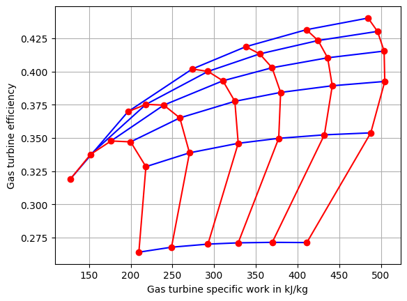
Make individual parameter variations for the compressor pressure ratio and the turbine inlet temperature:
Calculate thermal efficiency for every combination of values.
Plot the thermal efficiency as function of the total power generated grouped by turbine inlet temperature and by the compressor pressure ratio.
Solution 5#
import numpy as np
import pandas as pd
nwk.save("tmp")
# parameter study: pressure ratio and expander inlet temperature

# create data ranges and frames
pr_range = np.array([5, 10, 15, 20, 25, 30])
temperature_range = np.array([900.0, 1000.0, 1110.0, 1200.0, 1300.0, 1400.0])
df_eta = pd.DataFrame(columns=pr_range)
df_swk = pd.DataFrame(columns=pr_range)

# update parameter, solve all cases, results to csv data
for T in temperature_range:
    eta = []
    swk = []

    for pr in pr_range:
        # update parameter
        cp.set_attr(pr=pr)
        c3.set_attr(T=T)

        # solve case
        if pr == pr_range[0]:
            nwk.solve(mode='design', init_path="tmp")
        else:
            nwk.solve(mode='design')

        # calculate efficiency
        eta.append(abs(power_output.P.val) / (c5.m.val_SI * dcc.fuels["CH4"]["LHV"]))
        # calculate specific work
        swk.append(abs(power_output.P.val) / 1e3 / c1.m.val)

    # results to csv data
    df_eta.loc[T] = eta
    df_swk.loc[T] = swk
Invalid value for Q_loss: Q_loss = 4.2292482643824125e-05 above maximum value (0) at component combustion chamber.
Invalid value for Q_loss: Q_loss = 6.321400376881955e-05 above maximum value (0) at component combustion chamber.
Invalid value for Q_loss: Q_loss = 6.48071336494997e-05 above maximum value (0) at component combustion chamber.
The pressure at inlet 1 is lower than the pressure at the outlet of component combustion chamber.
Invalid value for Q_loss: Q_loss = 7.521793165084119e-05 above maximum value (0) at component combustion chamber.
The pressure at inlet 1 is lower than the pressure at the outlet of component combustion chamber.
Invalid value for Q_loss: Q_loss = 8.121583027226461e-05 above maximum value (0) at component combustion chamber.
The pressure at inlet 1 is lower than the pressure at the outlet of component combustion chamber.
Invalid value for Q_loss: Q_loss = 0.00011204287077050947 above maximum value (0) at component combustion chamber.
The pressure at inlet 1 is lower than the pressure at the outlet of component combustion chamber.
Invalid value for Q_loss: Q_loss = 0.00018007331989184903 above maximum value (0) at component combustion chamber.
The pressure at inlet 1 is lower than the pressure at the outlet of component combustion chamber.
Invalid value for Q_loss: Q_loss = 0.00017136996445573616 above maximum value (0) at component combustion chamber.
The pressure at inlet 1 is lower than the pressure at the outlet of component combustion chamber.
Invalid value for Q_loss: Q_loss = 0.00011542567261378485 above maximum value (0) at component combustion chamber.
The pressure at inlet 1 is lower than the pressure at the outlet of component combustion chamber.
Invalid value for Q_loss: Q_loss = 0.00012111626929505344 above maximum value (0) at component combustion chamber.
The pressure at inlet 1 is lower than the pressure at the outlet of component combustion chamber.
Invalid value for Q_loss: Q_loss = 0.00013851090146621732 above maximum value (0) at component combustion chamber.
The pressure at inlet 1 is lower than the pressure at the outlet of component combustion chamber.
Invalid value for Q_loss: Q_loss = 0.0001741482190160161 above maximum value (0) at component combustion chamber.
The pressure at inlet 1 is lower than the pressure at the outlet of component combustion chamber.
Invalid value for Q_loss: Q_loss = 0.00027469036030328706 above maximum value (0) at component combustion chamber.
The pressure at inlet 1 is lower than the pressure at the outlet of component combustion chamber.
Invalid value for Q_loss: Q_loss = 0.00021081250122632295 above maximum value (0) at component combustion chamber.
The pressure at inlet 1 is lower than the pressure at the outlet of component combustion chamber.
Invalid value for Q_loss: Q_loss = 0.0001597752205431123 above maximum value (0) at component combustion chamber.
The pressure at inlet 1 is lower than the pressure at the outlet of component combustion chamber.
Invalid value for Q_loss: Q_loss = 0.00012598516538635764 above maximum value (0) at component combustion chamber.
The pressure at inlet 1 is lower than the pressure at the outlet of component combustion chamber.
Invalid value for Q_loss: Q_loss = 0.00011893430992856992 above maximum value (0) at component combustion chamber.
The pressure at inlet 1 is lower than the pressure at the outlet of component combustion chamber.
Invalid value for Q_loss: Q_loss = 0.00013828540246890915 above maximum value (0) at component combustion chamber.
The pressure at inlet 1 is lower than the pressure at the outlet of component combustion chamber.
Invalid value for Q_loss: Q_loss = 0.0002222820255009037 above maximum value (0) at component combustion chamber.
The pressure at inlet 1 is lower than the pressure at the outlet of component combustion chamber.
Invalid value for Q_loss: Q_loss = 0.00014761065692400066 above maximum value (0) at component combustion chamber.
The pressure at inlet 1 is lower than the pressure at the outlet of component combustion chamber.
Invalid value for Q_loss: Q_loss = 9.874843251394794e-05 above maximum value (0) at component combustion chamber.
The pressure at inlet 1 is lower than the pressure at the outlet of component combustion chamber.
Invalid value for Q_loss: Q_loss = 8.962172748556719e-05 above maximum value (0) at component combustion chamber.
The pressure at inlet 1 is lower than the pressure at the outlet of component combustion chamber.
Invalid value for Q_loss: Q_loss = 2.0685961086771917e-05 above maximum value (0) at component combustion chamber.
The pressure at inlet 1 is lower than the pressure at the outlet of component combustion chamber.
The pressure at inlet 1 is lower than the pressure at the outlet of component combustion chamber.
The pressure at inlet 1 is lower than the pressure at the outlet of component combustion chamber.
The pressure at inlet 1 is lower than the pressure at the outlet of component combustion chamber.
The pressure at inlet 1 is lower than the pressure at the outlet of component combustion chamber.
The pressure at inlet 1 is lower than the pressure at the outlet of component combustion chamber.
The pressure at inlet 1 is lower than the pressure at the outlet of component combustion chamber.
The pressure at inlet 1 is lower than the pressure at the outlet of component combustion chamber.
The pressure at inlet 1 is lower than the pressure at the outlet of component combustion chamber.
The pressure at inlet 1 is lower than the pressure at the outlet of component combustion chamber.
The pressure at inlet 1 is lower than the pressure at the outlet of component combustion chamber.
The pressure at inlet 1 is lower than the pressure at the outlet of component combustion chamber.
The pressure at inlet 1 is lower than the pressure at the outlet of component combustion chamber.
Invalid value for Q_loss: Q_loss = 1.0592062803486835e-05 above maximum value (0) at component combustion chamber.
from matplotlib import pyplot as plt


fig, ax = plt.subplots(1)

for pr in pr_range:
    ax.plot(df_swk[pr], df_eta[pr], "b-")

for T in temperature_range:
    ax.plot(df_swk.loc[T], df_eta.loc[T], "ro-")

ax.set_ylabel("Gas turbine efficiency")
ax.set_xlabel("Gas turbine specific work in kJ/kg")
ax.grid()
ax.set_axisbelow(True)